2.5.2. Dynamic Systems Library (DynSysLib)

This page provides a summary of the Python Dynamical Systems Library (DynSysLib) for simulating a wide variety of dynamical systems. Full documentation of all of the currently available dynamical systems can be downloaded here.

Figure: x-solution to simulated rossler system for a chaotic response.

teaspoon.MakeData.DynSysLib.DynSysLib.DynamicSystems(system, dynamic_state=None, L=None, fs=None, SampleSize=None, parameters=None, InitialConditions=None, UserGuide=False)[source]

This function provides a library of dynamical system models to simulate with the time series as the output.

Parameters:

system (string) – either ‘periodic’ or ‘chaotic’.
dynamic_state (Optional[string]) – either ‘periodic’ or ‘chaotic’.
L (Optional[int]) – amount of time to solve simulation for.
fs (Optional[int]) – sampling rate for simulation.
SampleSize (Optional[int]) – length of sample at end of entire time series
parameters (Optional[array]) – dynamic system parameters.
InitialConditions (Optional[array]) – initial conditions for simulation.
UserGuide (Optional[bool]) –

Returns:

Array of the time indices as t and the simulation time series ts from the simulation for all dimensions of dynamcal system (e.g. 3 for Lorenz).

Return type:

array

Of the optional other parameters either the dynamic_state parameter or the system parameters must be used.

This function requires the following packages:

numpy
scipy
matplotlib
ddeint (delayed differential equations only)

2.5.2.1. Available Dynamical Systems

The following table provides a list of all the available dynamical systems as called by the system keyword:

Table 2.1 Available Dynmical Systems
Maps	Autonomous Dissipative Flows	Driven Dissipative Flows	Conservative Flows	Periodic Functions	Noise Models	Human Data	Delayed Flows
logistic_map	chua	driven_pendulum	driven_van_der_pol_oscillator	sine	gaussian_noise	ECG	mackey_glass
henon_map	lorenz	shaw_van_der_pol_oscillator	simplest_driven_chaotic_flow	incommensurate_sine	uniform_noise	EEG
logistic_map	rossler	forced_brusselator	nose_hoover_oscillator	rayleigh_noise
sine_map	coupled_lorenz_rossler	ueda_oscillator	labyrinth_chaos	exponential_noise
tent_map	coupled_rossler_rossler	duffings_two_well_oscillator	henon_heiles_system
linear_congruential_generator_map	double_pendulum	duffing_van_der_pol_oscillator
rickers_population_map	diffusionless_lorenz_attractor	rayleigh_duffing_oscillator
gauss_map	complex_butterfly
cusp_map	chens_system
pinchers_map	hadley_circulation
sine_circle_map	ACT_attractor
lozi_map	rabinovich_frabrikant_attractor
delayed_logstic_map	linear_feedback_rigid_body_motion_system
tinkerbell_map	moore_spiegel_oscillator
burgers_map	thomas_cyclically_symmetric_attractor
holmes_cubic_map	halvorsens_cyclically_symmetric_attractor
kaplan_yorke_map	burke_shaw_attractor
	rucklidge_attractor
	WINDMI
	simplest_quadratic_chaotic_flow
	simplest_cubic_chaotic_flow
	simplest_piecewise_linear_chaotic_flow
	double_scroll

2.5.2.2. Examples

The following is an example implementing the minimum amount of needed:

import matplotlib.pyplot as plt
import matplotlib.gridspec as gridspec
import teaspoon.MakeData.DynSysLib.DynSysLib as DSL

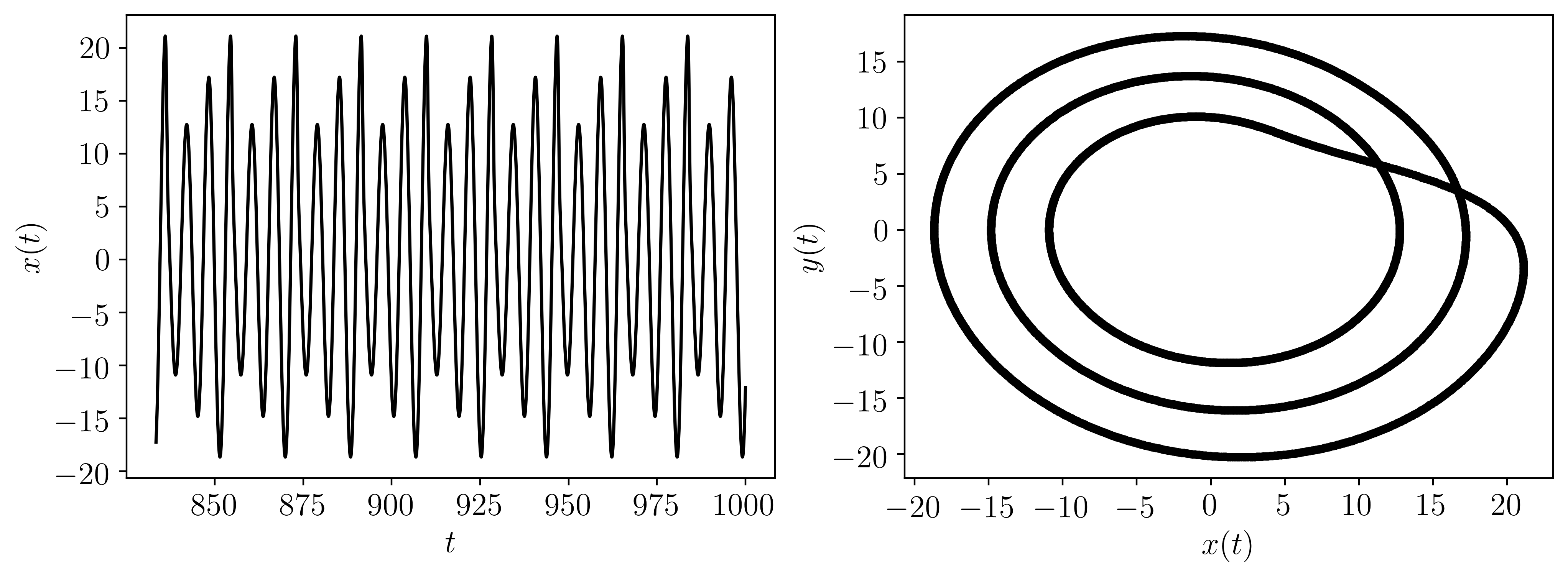
system = 'rossler'
dynamic_state = 'periodic'
t, ts = DSL.DynamicSystems(system, dynamic_state)

TextSize = 15
plt.figure(figsize = (12,4))
gs = gridspec.GridSpec(1,2)

ax = plt.subplot(gs[0, 0])
plt.xticks(size = TextSize)
plt.yticks(size = TextSize)
plt.ylabel(r'$x(t)$', size = TextSize)
plt.xlabel(r'$t$', size = TextSize)
plt.plot(t,ts[0], 'k')

ax = plt.subplot(gs[0, 1])
plt.plot(ts[0], ts[1],'k.')
plt.plot(ts[0], ts[1],'k', alpha = 0.25)
plt.xticks(size = TextSize)
plt.yticks(size = TextSize)
plt.xlabel(r'$x(t)$', size = TextSize)
plt.ylabel(r'$y(t)$', size = TextSize)

plt.show()

Where the output for this example is:

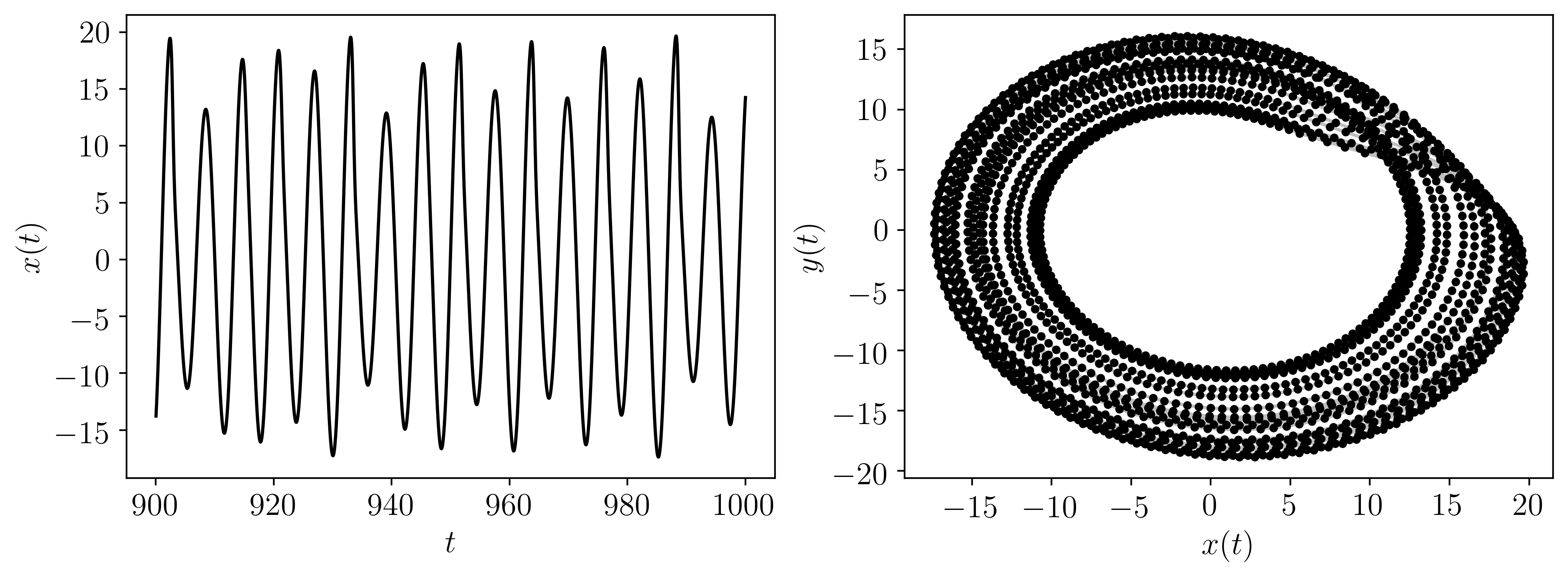
The following is another example implementing all of the possible inputs (dynamic_state is not needed when parameters are provided):

import matplotlib.pyplot as plt
import matplotlib.gridspec as gridspec
import teaspoon.MakeData.DynSysLib.DynSysLib as DSL

system = 'rossler'
UserGuide = True
L, fs, SampleSize = 1000, 20, 2000
# the length (in seconds) of the time series, the sample rate, and the sample size of the time series of the simulated system.
parameters = [0.1, 0.2, 13.0] # these are the a, b, and c parameters from the Rossler system model.
InitialConditions = [1.0, 0.0, 0.0] # [x_0, y_0, x_0]
t, ts = DSL.DynamicSystems(system, dynamic_state, L, fs, SampleSize, parameters,  InitialConditions, UserGuide)

TextSize = 15
plt.figure(figsize = (12,4))
gs = gridspec.GridSpec(1,2)

ax = plt.subplot(gs[0, 0])
plt.xticks(size = TextSize)
plt.yticks(size = TextSize)
plt.ylabel(r'$x(t)$', size = TextSize)
plt.xlabel(r'$t$', size = TextSize)
plt.plot(t,ts[0], 'k')

ax = plt.subplot(gs[0, 1])
plt.plot(ts[0], ts[1],'k.')
plt.plot(ts[0], ts[1],'k', alpha = 0.25)
plt.xticks(size = TextSize)
plt.yticks(size = TextSize)
plt.xlabel(r'$x(t)$', size = TextSize)
plt.ylabel(r'$y(t)$', size = TextSize)

plt.show()

Where the output for this example is:

Additionally, the user guide was prompted by setting UserGuide = True, which provides some simple instructions and a list of all the current systems:

----------------------------------------User Guide----------------------------------------------

This code outputs a time array t and a list time series for each variable of the dynamic system.
The user is only required to enter the system (see list below) as a string and
the dynamic state as either periodic or chaotic as a string.

The user also has the optional inputs as the time series length in seconds (L),
the sampling rate (fs), and the sample size (SampleSize).
If the user does not supply these values, they are defaulted to preset values.

Other optional inputs are parameters and InitialConditions. The parameters variable
needs to be entered as a list or array and are the dynamic system parameters.
If the correct number of parameters is not provided it will default to preset parameters.
The InitialConditions variable is also a list or array and is the initial conditions of the system.
The length of the initial conditions also need to match the system being analyzed.

List of the dynamic systems available:
___________________
Maps:
-------------------
1 : logistic_map
2 : henon_map
3 : sine_map
4 : tent_map
5 : linear_congruential_generator_map
6 : rickers_population_map
7 : gauss_map
8 : cusp_map
9 : pinchers_map
10 : sine_circle_map
11 : lozi_map
12 : delayed_logstic_map
13 : tinkerbell_map
14 : burgers_map
15 : holmes_cubic_map
16 : kaplan_yorke_map
___________________


___________________
Autonomous Dissipative Flows:
-------------------
1 : chua
2 : lorenz
3 : rossler
4 : coupled_lorenz_rossler
5 : coupled_rossler_rossler
6 : double_pendulum
7 : diffusionless_lorenz_attractor
8 : complex_butterfly
9 : chens_system
10 : hadley_circulation
11 : ACT_attractor
12 : rabinovich_frabrikant_attractor
13 : linear_feedback_rigid_body_motion_system
14 : moore_spiegel_oscillator
15 : thomas_cyclically_symmetric_attractor
16 : halvorsens_cyclically_symmetric_attractor
17 : burke_shaw_attractor
18 : rucklidge_attractor
19 : WINDMI
20 : simplest_quadratic_chaotic_flow
21 : simplest_cubic_chaotic_flow
22 : simplest_piecewise_linear_chaotic_flow
23 : double_scroll
___________________


___________________
Driven Dissipative Flows:
-------------------
1 : driven_pendulum
2 : driven_can_der_pol_oscillator
3 : shaw_van_der_pol_oscillator
4 : forced_brusselator
5 : ueda_oscillator
6 : duffings_two_well_oscillator
7 : duffing_van_der_pol_oscillator
8 : rayleigh_duffing_oscillator
___________________


___________________
Conservative Flows:
-------------------
1 : simplest_driven_chaotic_flow
2 : nose_hoover_oscillator
3 : labyrinth_chaos
4 : henon_heiles_system
___________________


___________________
Periodic Functions:
-------------------
1 : sine
2 : incommensurate_sine
___________________


___________________
Noise Models:
-------------------
1 : gaussian_noise
2 : uniform_noise
3 : rayleigh_noise
4 : exponential_noise
___________________


___________________
Human Data:
-------------------
1 : ECG
2 : EEG
___________________


___________________
Delayed Flows:
-------------------
1 : mackey_glass
___________________

------------------------------------------------------------------------------------------------