2.4.3. Information Module

This page provides a summary of the functions available in the information module.

Currently, the following functions are available:

Permutation Entropy
Multi-scale Permutation Entropy
Persistent Entropy

2.4.3.1. Entropy

One of the most common ways to represent information from a data source is through the measurement of entropy. In this sub-module we have included some implementations of measuring entropy from a signal (permutation entropy) and persistence diagram (persistent entropy). Entropy is calculated as

\[h = -\sum_{x \in X} p(x) {\rm log}_2(p(x),\]

where p(x) is the probability of data type x, which is an element of the finite set of data types X. Additional, the log is base 2 so that the entropy as units of information. Persistent entropy is normalized on a scale from [0,1] with no units as

\[h' = \frac{h}{\# \{ x \in X \} },\]

where # denotes the number of data types in X.

2.4.3.1.1. Permutation Entropy

Permutation entropy uses the data types of permutations (see Permutation Sequence Generation for details on permutations) and calculates the probability of each as their respective occurance in a time series.

teaspoon.SP.information.entropy.PE(ts, n=5, tau=10, normalize=False)[source]

This function takes a time series and calculates Permutation Entropy (PE).

Parameters:

ts (array) – Time series (1d).
n (int) – Permutation dimension. Default is 5.
tau (int) – Permutation delay. Default is 10.

Kwargs:: normalize (bool): Normalizes the permutation entropy on scale from 0 to 1. defaut is False.

Returns:: PE, the permutation entropy.
Return type:: (float)

Example:

import numpy as np
t = np.linspace(0,100,2000)
ts = np.sin(t)  #generate a simple time series

from teaspoon.SP.information.entropy import PE
h = PE(ts, n = 6, tau = 15, normalize = True)
print('Permutation entropy: ', h)

Output of example:

Permutation entropy:  0.4350397222113192

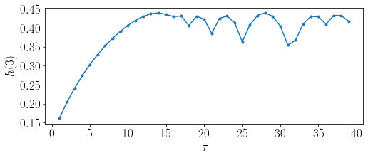
2.4.3.1.2. Multi-scale Permutation Entropy

Multi-scale Permutation Entropy applies the permutation entropy calculation over multiple time scales (delays).

teaspoon.SP.information.entropy.MsPE(ts, n=5, delay_end=200, plotting=False, normalize=False)[source]

This function takes a time series and calculates Multi-scale Permutation Entropy (MsPE): over multiple time scales

Parameters:

ts (array) – Time series (1d).
n (int) – Permutation dimension. Default is 5.
delay_end (int) – maximum delay in search. default is 200.

Kwargs:: plotting (bool): Plotting for user interpretation. defaut is False. normalize (bool): Normalizes the permutation entropy on scale from 0 to 1. defaut is False.

Returns:: MsPE, the permutation entropy over multiple time scales.
Return type:: (array)

Example:

import numpy as np
t = np.linspace(0,100,2000)
ts = np.sin(t)  #generate a simple time series

from teaspoon.SP.information.entropy import MsPE
delays,H = MsPE(ts, n = 6, delay_end = 40, normalize = True)

import matplotlib.pyplot as plt
plt.figure(2)
TextSize = 17
plt.figure(figsize=(8,3))
plt.plot(delays, H, marker = '.')
plt.xticks(size = TextSize)
plt.yticks(size = TextSize)
plt.ylabel(r'$h(3)$', size = TextSize)
plt.xlabel(r'$\tau$', size = TextSize)
plt.show()

Output of example:

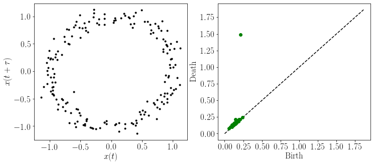
2.4.3.1.3. Persistent Entropy

Persistent entropy uses the data types of lifetimes from a persistence diagram and calculates their respective probability as

\[p(\ell) = \frac{\ell}{\sum_{\ell \in L}\ell},\]

where L is the set of lifetimes.

teaspoon.SP.information.entropy.PersistentEntropy(lifetimes, normalize=False)[source]

This function takes a time series and calculates Permutation Entropy (PE).

Parameters:: lifetimes (array) – Lifetimes from persistence diagram (1d).

Kwargs:: normalize (bool): Normalizes the entropy on scale from 0 to 1. defaut is False.

Returns:: PerEn, the persistence diagram entropy.
Return type:: (float)

Example:

import numpy as np
#generate a simple time series with noise
t = np.linspace(0,20,200)
ts = np.sin(t) +np.random.normal(0,0.1,len(t))

from teaspoon.SP.tsa_tools import takens
#embed the time series into 2 dimension space using takens embedding
embedded_ts = takens(ts, n = 2, tau = 15)

from ripser import ripser
#calculate the rips filtration persistent homology
result = ripser(embedded_ts, maxdim=1)
diagram = result['dgms']

#--------------------Plot embedding and persistence diagram---------------
import matplotlib.pyplot as plt
import matplotlib.gridspec as gridspec
gs = gridspec.GridSpec(1, 2)
plt.figure(figsize = (12,5))
TextSize = 17
MS = 4

ax = plt.subplot(gs[0, 0])
plt.yticks( size = TextSize)
plt.xticks(size = TextSize)
plt.xlabel(r'$x(t)$', size = TextSize)
plt.ylabel(r'$x(t+\tau)$', size = TextSize)
plt.plot(embedded_ts.T[0], embedded_ts.T[1], 'k.')

ax = plt.subplot(gs[0, 1])
top = max(diagram[1].T[1])
plt.plot([0,top*1.25],[0,top*1.25],'k--')
plt.yticks( size = TextSize)
plt.xticks(size = TextSize)
plt.xlabel('Birth', size = TextSize)
plt.ylabel('Death', size = TextSize)
plt.plot(diagram[1].T[0],diagram[1].T[1] ,'go', markersize = MS+2)

plt.show()
#-------------------------------------------------------------------------

#get lifetimes (L) as difference between birth (B) and death (D) times
B, D = diagram[1].T[0], diagram[1].T[1]
L = D - B

from teaspoon.SP.information.entropy import PersistentEntropy
h = PersistentEntropy(lifetimes = L)

print('Persistent entropy: ', h)

Output of example:

Persistent entropy:  1.7693450019916783