2.3.1. Persistent Homology of Networks (PHN)

This page provides a summary of the python functions used in “Persistent Homology of Complex Networks for Dynamic State Detection” for generating and analyzing complex networks as the Persistent Homology of Networks (PHN). Additionally, a basic example is provided showing the functionality of the method for a simple time series. Below, a simple overview of the method is provided.

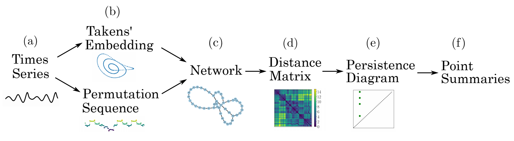
Outline of method: a time series (a) is embedded (b) using state space reconstruction from Takens’ embedding or segmenting the vectors into a set of permutations. From these two representations, an undirected, unweighted network (c) is formed by either applying a kth nearest neighbors algorithm or by setting each permutation state as a node. The distance matrix (d) is calculated using the shortest path between all nodes. The persistence diagram (e) is generated by applying persistent homology to the distance matrix. Finally, one of several point summaries (f) are used to extract information from the persistence diagram.

teaspoon.TDA.PHN.DistanceMatrix(A, method='shortest_unweighted_path')

This function calculates the distance matrix from a connected graph represented as an adjacency matrix using an available method.”

Parameters:

• A (2-D array) – 2-D square adjacency matrix

• method (str) – Method for calculating distances between nodes. default is shortest_unweighted_path. Options are shortest_unweighted_path, shortest_weighted_path, weighted_shortest_path, and diffusion_distance.

Returns:

Distance matrix between all node pairs.

Return type:

[2-D array]

teaspoon.TDA.PHN.PH_network(D, max_homology_dimension=1)

This function calculates the persistent homology of the graph represented by the adjacency matrix A using a distance algorithm defined by user.

Parameters:

• D (2-D array) – Distance matrix between all node pairs.

• max_homology_dimension (Optional[int]) – maximum dimension of the homology.

Returns:

list of lists where ech list is a persistence diagram (standard ripser format).

Return type:

[list]

teaspoon.TDA.PHN.point_summaries(diagram, A)

This function calculates the persistent homology statistics for a graph from the paper “Persistent Homology of Complex Networks for Dynamic State Detection.”

Parameters:

• A (2-D array) – 2-D square adjacency matrix

• diagram (list) – persistence diagram from ripser from a graph’s distance matrix

Returns:

statistics (R, En M) as (maximum persistence ratio, persistent entropy normalized, homology class ratio). Returns NaNs if empty diagram.

Return type:

[array 1-D]

2.3.1.1. Example

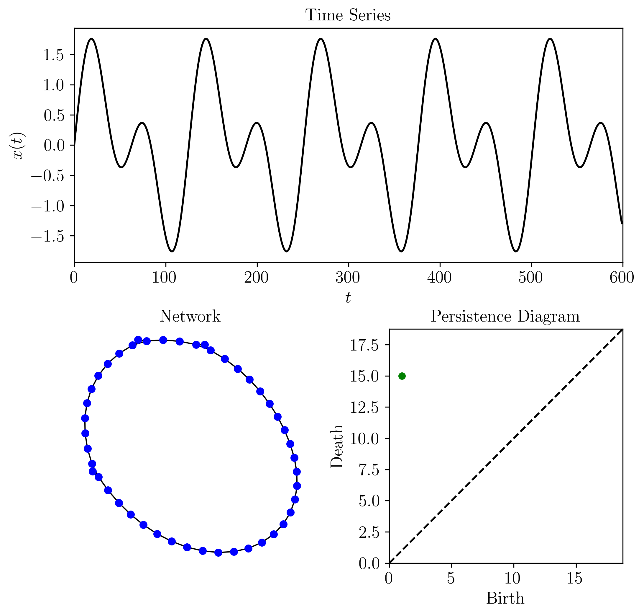
The following is an example implementing the method for an ordinal partition network and shortest unweighted path distance for a simple periodic time series. However, other network types (e.g., k-NN or CGSSN) could be used and other distances (e.g., weighted shortest path or diffusion distance) could have been used. These other distances and networks are described in the signal processing module.:

#import needed packages
import numpy as np
import matplotlib.pyplot as plt
import matplotlib.gridspec as gridspec
import networkx as nx

#teaspoon functions
from teaspoon.SP.network import ordinal_partition_graph
from teaspoon.SP.network_tools import remove_zeros
from teaspoon.SP.network_tools import make_network
from teaspoon.TDA.PHN import DistanceMatrix, point_summaries, PH_network

# Time series data
t = np.linspace(0,30,600)
ts = np.sin(t) + np.sin(2*t) #generate a simple time series

A = ordinal_partition_graph(ts, n = 6) #adjacency matrix
A = remove_zeros(A) #remove nodes of unused permutation
G = nx.from_numpy_matrix(A)
G.remove_edges_from(nx.selfloop_edges(G))
#create distance matrix and calculate persistence diagram
D = DistanceMatrix(A, method = 'diffusion_distance')
diagram = PH_network(D)

print('1-D Persistent Homology (loops): ', diagram[1])

stats = point_summaries(diagram, A)
print('Persistent homology of network statistics: ', stats)



TextSize = 14
plt.figure(2)
plt.figure(figsize=(8,8))
gs = gridspec.GridSpec(4, 2)

ax = plt.subplot(gs[0:2, 0:2]) #plot time series
plt.title('Time Series', size = TextSize)
plt.plot(ts, 'k')
plt.xticks(size = TextSize)
plt.yticks(size = TextSize)
plt.xlabel('$t$', size = TextSize)
plt.ylabel('$x(t)$', size = TextSize)
plt.xlim(0,len(ts))

ax = plt.subplot(gs[2:4, 0])
plt.title('Network', size = TextSize)
nx.draw(G, with_labels=False, font_weight='bold', node_color='blue',
    width=1, font_size = 10, node_size = 30)

ax = plt.subplot(gs[2:4, 1])
plt.title('Persistence Diagram', size = TextSize)
MS = 3
top = max(diagram[1].T[1])
plt.plot([0,top*1.25],[0,top*1.25],'k--')
plt.yticks( size = TextSize)
plt.xticks(size = TextSize)
plt.xlabel('Birth', size = TextSize)
plt.ylabel('Death', size = TextSize)
plt.plot(diagram[1].T[0],diagram[1].T[1] ,'go', markersize = MS+2)
plt.xlim(0,top*1.25)
plt.ylim(0,top*1.25)

plt.subplots_adjust(hspace= 0.8)
plt.subplots_adjust(wspace= 0.35)
plt.show()

Where the output for this example is:

1-D Persistent Homology (loops):  [[ 1. 15.]]
Persistent homology of network statistics:  [0.0, 0, 0.02127659574468085]