2.4.2. Network Representation of Time Series

This module provides algorithms for forming both ordinal partition networks (see example GIF below) and k-NN networks. The formation of the networks is described in detail in “Persistent Homology of Complex Networks for Dynamic State Detection.”

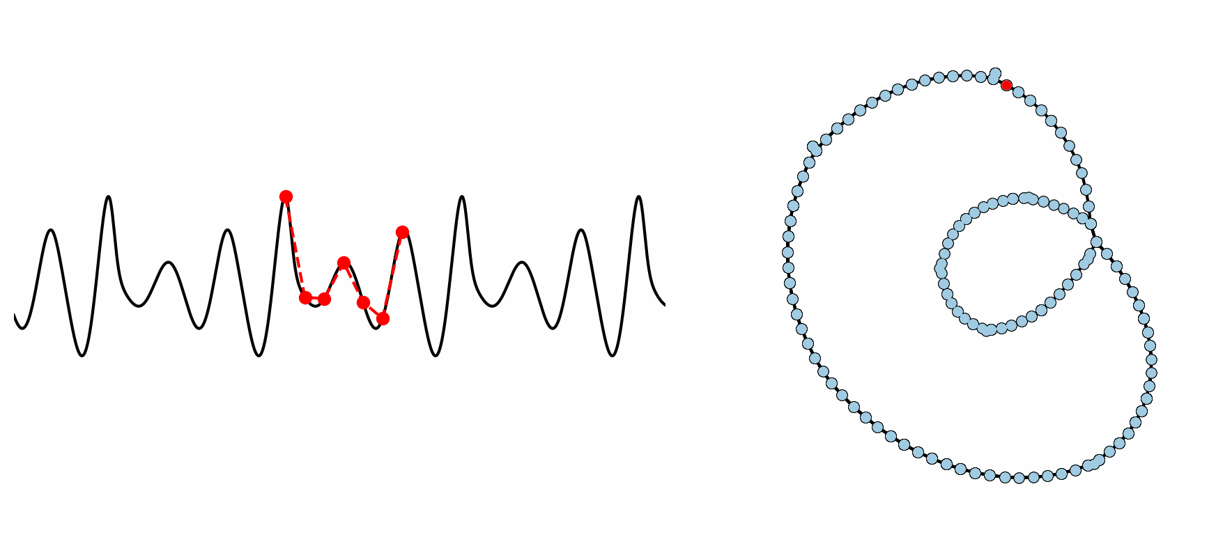
Figure: Example formation of an ordinal partition network for 6 dimensional permutations. As the ordinal ranking of the 6 spaced points changes, so does the node in the network. This shows how the network captures the periodic structure of the time series through a resulting double loop topology.

2.4.2.1. k Nearest Neighbors Graph

teaspoon.SP.network.Adjacency_KNN(indices)[source]

This function takes the indices of nearest neighbors and creates an adjacency matrix.

Parameters:: indices (array of ints) – array of arrays of indices of n nearest neighbors.
Returns:: Adjacency matrix
Return type:: [A]

teaspoon.SP.network.knn_graph(ts, n=None, tau=None, k=4)[source]

This function creates an k-NN network represented as an adjacency matrix A using a 1-D time series

Parameters:

ts (1-D array) – 1-D time series signal
n (Optional[int]) – embedding dimension for state space reconstruction. Default is uses FNN algorithm from parameter_selection module.
tau (Optional[int]) – embedding delay fro state space reconstruction. Default uses MI algorithm from parameter_selection module.
k (Optional[int]) – number of nearest neighbors for graph formation.

Returns:

A (2-D weighted and directed square adjacency matrix)

Return type:

[2-D square array]

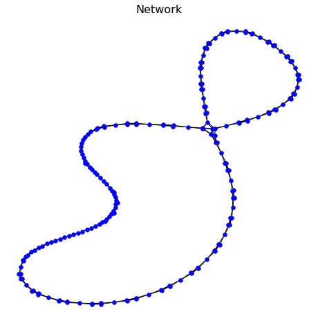
The network output has the data structure of an adjacency matrix (or networkx graph for displaying). An example is shown below:

#import needed packages
import numpy as np
import matplotlib.pyplot as plt
import networkx as nx
from teaspoon.SP.network import knn_graph
from teaspoon.SP.network_tools import make_network

# Time series data
t = np.linspace(0,30,200)
ts = np.sin(t) + np.sin(2*t) #generate a simple time series

A = knn_graph(ts) #adjacency matrix

G, pos = make_network(A) #get networkx representation

plt.figure(figsize = (8,8))
plt.title('Network', size = 16)
nx.draw(G, pos, with_labels=False, font_weight='bold', node_color='blue',
        width=1, font_size = 10, node_size = 30)
plt.show()

This code has the output as follows:

2.4.2.2. Ordinal Partition Graph

teaspoon.SP.network.Adjaceny_OP(perm_seq, n)[source]

This function takes the permutation sequence and creates a weighted and directed adjacency matrix.

Parameters:

perm_seq (array of ints) – array of the permutations (chronologically ordered) that were visited.
n (int) – dimension of permutations.

Returns:

Adjacency matrix

Return type:

[A]

teaspoon.SP.network.ordinal_partition_graph(ts, n=None, tau=None)[source]

This function creates an ordinal partition network represented as an adjacency matrix A using a 1-D time series

Parameters:

ts (1-D array) – 1-D time series signal
n (Optional[int]) – embedding dimension for state space reconstruction. Default is uses MsPE algorithm from parameter_selection module.
tau (Optional[int]) – embedding delay fro state space reconstruction. Default uses MsPE algorithm from parameter_selection module.

Returns:

A (2-D weighted and directed square adjacency matrix)

Return type:

[2-D square array]

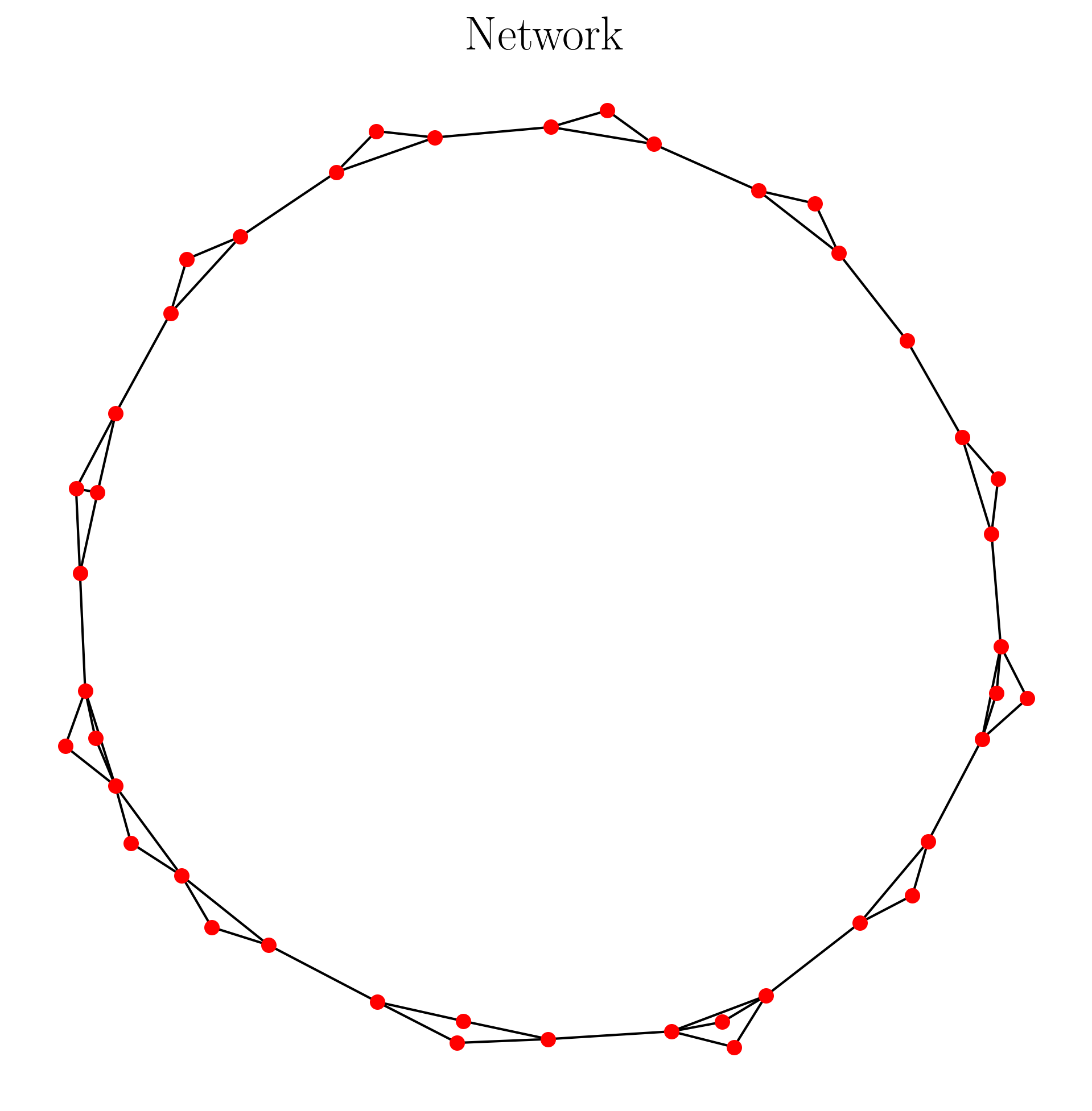
The network output has the data structure of an adjacency matrix (or networkx graph for displaying). An example is shown below:

#import needed packages
import numpy as np
import matplotlib.pyplot as plt
import networkx as nx
#teaspoon functions
from teaspoon.SP.network import ordinal_partition_graph
from teaspoon.SP.network_tools import remove_zeros
from teaspoon.SP.network_tools import make_network

# Time series data
t = np.linspace(0,30,200)
ts = np.sin(t) + np.sin(2*t) #generate a simple time series

A = ordinal_partition_graph(ts, n = 6) #adjacency matrix
A = remove_zeros(A) #remove nodes of unused permutation

G, pos = make_network(A) #get networkx representation

plt.figure(figsize = (8,8))
plt.title('Network', size = 20)
nx.draw(G, pos, with_labels=False, font_weight='bold', node_color='red',
        width=1, font_size = 10, node_size = 30)
plt.show()

This code has the output as follows:

2.4.2.3. Coarse Grained State Space (CGSS) Graph

teaspoon.SP.network.Adjacency_CGSS(state_seq, N=None, delay=1)[source]

This function takes the CGSS state sequence and creates a weighted and directed adjacency matrix.

Parameters:

state_seq (array of ints) – array of the states visited in SSR (chronologically ordered).
N (int) – dnumber of total possible states.

Returns:

Adjacency matrix

Return type:

[A]

teaspoon.SP.network.cgss_graph(ts, B_array, n=None, tau=None)[source]

This function creates a coarse grained state space network (CGSSN) represented as an adjacency matrix A using a 1-D time series and binning array.

Parameters:

ts (1-D array) – 1-D time series signal
B_array (1-D array) – array of bin edges for binning SSR for each dimension.
n (Optional[int]) – embedding dimension for state space reconstruction. Default is uses MsPE algorithm from parameter_selection module.
tau (Optional[int]) – embedding delay fro state space reconstruction. Default uses MsPE algorithm from parameter_selection module.

Returns:

A (2-D weighted and directed square adjacency matrix)

Return type:

[2-D square array]

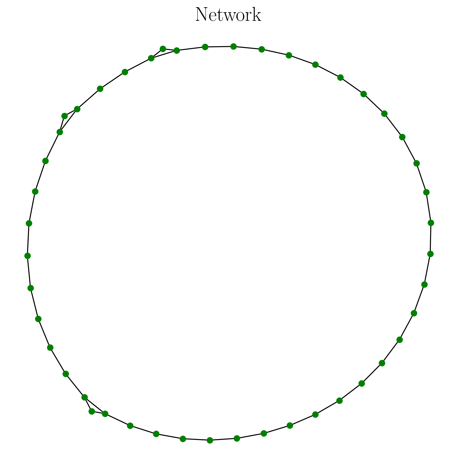
The network output has the data structure of an adjacency matrix (or networkx graph for displaying). An example is shown below:

#import needed packages
import numpy as np
import matplotlib.pyplot as plt
import networkx as nx
#teaspoon functions
from teaspoon.SP.network import cgss_graph
from teaspoon.SP.network_tools import remove_zeros
from teaspoon.SP.network_tools import make_network
from teaspoon.parameter_selection import MsPE
import teaspoon.SP.tsa_tools as tsa_tools

# Time series data
t = np.linspace(0,30,600)
ts = np.sin(t) + np.sin(2*t) #generate a simple time series

n = 3 #dimension of SSR
b = 8 #number of states per dimension
tau = MsPE.MsPE_tau(ts)

B_array = tsa_tools.cgss_binning(ts, n, tau, b) #binning array
SSR = tsa_tools.takens(ts, n, tau)  #state space reconstruction

A = cgss_graph(ts, B_array, n, tau) #adjacency matrix
A = remove_zeros(A) #remove nodes of unused permutation

G, pos = make_network(A) #get networkx representation

plt.figure(figsize = (8,8))
plt.title('Network', size = 20)
nx.draw(G, pos, with_labels=False, font_weight='bold', node_color='green',
        width=1, font_size = 10, node_size = 30)
plt.show()

This code has the output as follows:

2.4.2.4. Network Tools

teaspoon.SP.network_tools.degree_matrix(A)[source]

This function calculates the degree matrix from theadjacency matrix. A degree matrix is an empty matrix with diagonal filled with degree vector.

Parameters:: A (2-D array) – adjacency matrix of single component graph.
Returns:: Degree matrix.
Return type:: [2-D array]

teaspoon.SP.network_tools.diffusion_distance(A, d, t, lazy=False)[source]

This function calculates the diffusion distance for t random walk steps.

Parameters:

A (matrix) – adjacency matrix of graph.
d (array) – degree vector
t (int) – random walk steps. Should be approximately twice the diameter of graph.
lazy (Optional[boolean]) – optional to use self transition probability (50%).

Returns:

A (2-D weighted and directed square probability transition matrix)

Return type:

[2-D square array]

teaspoon.SP.network_tools.make_network(A, position_iterations=1000, remove_deg_zero_nodes=False)[source]

This function creates a networkx graph and position of the nodes using the adjacency matrix.

Parameters:

A (2-D array) – 2-D square adjacency matrix
position_iterations (Optional[int]) – Number of spring layout position iterations. Default is 1000.

Returns:

G (networkx graph representation), pos (position of nodes for networkx drawing)

Return type:

[dictionaries, list]

teaspoon.SP.network_tools.random_walk(A, lazy=False)[source]

This function calculates the 1 step random walk probability matrix using the adjacency matrix.

Parameters:

A (matrix) – adjacency matrix of graph.
lazy (Optional[boolean]) – optional to use self transition probability (50%).

Returns:

A (2-D weighted and directed square probability transition matrix)

Return type:

[2-D square array]

teaspoon.SP.network_tools.remove_zeros(A)[source]

This function removes unused vertices from adjacency matrix.

Parameters:: A (matrix) – 2-D weighted and directed square probability transition matrix

Returns: [2D matrix]: 2-D weighted and directed square probability transition matrix

teaspoon.SP.network_tools.shortest_path(A, weighted_path_lengths=False)[source]

This function calculates the shortest path distance matrix for a signal component graph represented as an adjacency matrix A.

Parameters:

A (2-D array) – adjacency matrix of single component graph.
n (Optional[int]) – option to calculate the shortest path between nodes using the inverse of the edge weights.

Returns:

Distance matrix of shortest path lengths between all node pairs.

Return type:

[2-D array]

teaspoon.SP.network_tools.visualize_network(A, position_iterations=1000, remove_deg_zero_nodes=False)[source]

This function creates a networkx graph and position of the nodes using the adjacency matrix.

Parameters:

A (2-D array) – 2-D square adjacency matrix
position_iterations (Optional[int]) – Number of spring layout position iterations. Default is 1000.

Returns:

G (networkx graph representation), pos (position of nodes for networkx drawing)

Return type:

[dictionaries, list]

teaspoon.SP.network_tools.weighted_shortest_path(A)[source]

This function calculates the weighted shortest path distance matrix for a signal component graph represented as an adjacency matrix A. The paths are found tusing the edge weights as the inverse of the adjacency matrix weight and the distance is the sum of the adjacency matrix weights along that path.

Parameters:: A (2-D array) – adjacency matrix of single component graph.
Returns:: Distance matrix of shortest path lengths between all node pairs.
Return type:: [2-D array]