2.4.5. Texture Analysis
This page provides a summary of the functions available in the texture analysis module. Persistent homology from topological data analysis is leveraged to compare experimental and nominal textures and provide similarity scores for specific features that make up the texture of interest. Three texture features were targeted for this module: lattice shape, feature depth, and roundness. More information on the details of texture shape quantification can be found in, “Topological Measures for Pattern quantification of Impact Centers in Piezo Vibration Striking Treatment (PVST).” The methods for feature depth and roundness are described in “Pattern Characterization Using Topological Data Analysis: Application to Piezo Vibration Striking Treatment.”
Currently, the following functions are available:
2.4.5.1. Texture Analaysis Overview
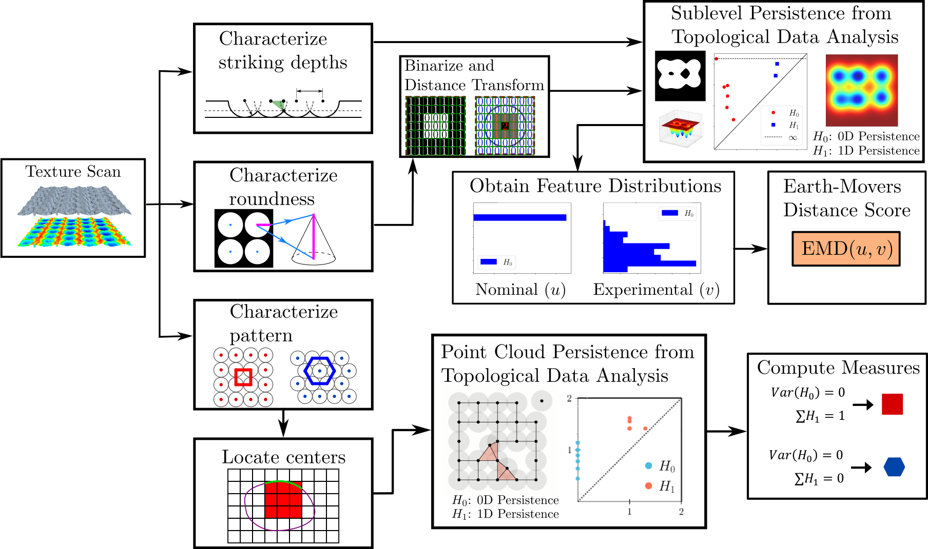
The process for analyzing these texture features is captured in the overview flow chart below.
2.4.5.1.1. Lattice Shape
Point cloud persistent homology is computed on the coordinates of the feature centers and the corresponding lattice shape scores are computed to extract lattice shape information from a texture.
- teaspoon.SP.texture_analysis.lattice_shape(data, plot=False)[source]
Quantify the lattice shape of a given point cloud of center points.
- Parameters:
data (array) – (x,y) strike center coordinates.
plot (bool) – Boolean variable to plot the persistence diagram and lifetime histogram
- Returns:
[varh0, sumh1] – Array containing the 0D and 1D persistence scores for the given point cloud
An example usage of this function is provided below where synthetic grids are generated to simulate the nominal and experimental feature center coordinates. The experimental grid has been perturbed by adding uniform noise to the x and y coordinates. The two input grids are shown in the figure below.

Example:
import numpy as np
from teaspoon.SP.texture_analysis import lattice_shape
np.random.seed(48824)
n = 10
x = np.linspace(-1, 1, n) + np.random.uniform(-0.1,0.1, n)
y = np.linspace(-1, 1, n) + np.random.uniform(-0.1,0.1, n)


xv, yv = np.meshgrid(x, y)
xv = xv.reshape(-1, 1)
yv = yv.reshape(-1, 1)

data = np.column_stack((xv, yv))
scores = lattice_shape(data)
Output of example:
Scores:
    [varh0, sumh1] = [0.01458, 0.65979]
2.4.5.1.2. Feature Depth
0D Sub level persistent homology is computed on nominal and experimental texture images, and the lifetime histograms are compared to provide a score based on the earth movers distance indicating the uniformity of the feature depths across the experimental image.
- teaspoon.SP.texture_analysis.feature_depth(nom_image, exp_image, nfeat, plot=False)[source]
Quantify the striking depths of a given texture scan.
- Parameters:
nom_image (array) – 2D image of the nominal surface (scaled between 0-1)
exp_image (array) – 2D image of the experimental surface (scaled between 0-1)
nfeat (int) – Expected number of features in the image
plot (bool) – Variable to plot the persistence diagram and lifetime histograms
- Returns:
depth_score – The earth movers distance score as a percentage
- Return type:
(float)
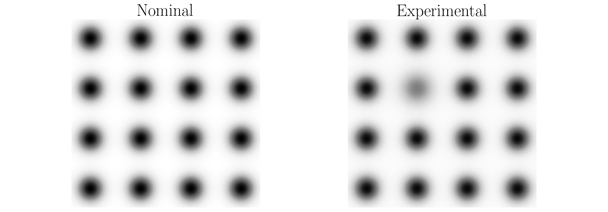
An example use of this function is provided below. The example generates synthetic surfaces representing the nominal and experimental textures. These generated surfaces are shown below where there are 16 features in each image generated using 2D Gaussian distributions. One of the features in the experimental image is shallower than the others representing a non uniform depth distribution. Further, samples from a Gaussian distribution are added to the experimental surface to introduce noise in the image and further alter the depth distribution.
Example:
import numpy as np
from scipy.stats import multivariate_normal
from teaspoon.SP.texture_analysis import feature_depth

# Generate a grid of sample xy pairs
n = 500
x = np.linspace(-1, 1, n)
y = np.linspace(-1, 1, n)
xv, yv = np.meshgrid(x, y)
xv = xv.reshape(-1, 1)
yv = yv.reshape(-1, 1)
xy = np.column_stack((xv, yv))
nom = 0
exp = 0
ind = 0

# Generate Grid of Strike Locations
grid_size = 4
xc = np.linspace(-0.8, 0.8, grid_size)
yc = np.linspace(-0.8, 0.8, grid_size)
xvc, yvc = np.meshgrid(xc, yc)
xvc = xvc.reshape(-1, 1)
yvc = yvc.reshape(-1, 1)
xyc = np.column_stack((xvc, yvc))


# Generate 3D surface from gaussian distribution and scale between 0-1
for point in xyc:
    ind += 1
    nom += multivariate_normal.pdf(xy, mean=np.array([point[0], point[1]]), cov=np.diag(np.array([0.1, 0.1]) ** 2))
    if ind == 6:
        exp += multivariate_normal.pdf(xy, mean=np.array([point[0], point[1]]), cov=np.diag(np.array([0.13, 0.13]) ** 2))
    else:
        exp += multivariate_normal.pdf(xy, mean=np.array([point[0], point[1]]), cov=np.diag(np.array([0.1, 0.1]) ** 2))

nom = nom.reshape(n, n).astype(np.float64)
nom = -1.0 * nom + np.max(nom)
nom = nom / np.max(nom) # scale between 0-1

exp = exp.reshape(n, n).astype(np.float64)
exp = -1.0 * exp + np.max(exp)
exp = exp / np.max(exp) # scale between 0-1


# Generate nominal and experimental images by adding noise and scaling from 0-1 again
np.random.seed(48824)
nom_im = nom
exp_im = exp + np.random.normal(scale=0.01, size=[n,n])
exp_im = (exp_im - np.min(exp_im))/(np.max(exp_im) - np.min(exp_im)) # Scale between 0-1

# Compute the depth score
score = feature_depth(nom_im, exp_im, 16, plot=False)
Output of example:
depth_score = 92.13
2.4.5.1.3. Feature Roundness
1D Sub level persistent homology is computed on nominal and experimental texture images. The images are thresholded at many heights and at each height the thresholded image is distance transformed to encode information about the roundness of the feature as the height function of the transormed image. 1D sub level persistence is then used to compare the histograms of the loop lifetimes at each height. An overall score is computed as the area under the earth movers distance curve normalized to the reference height of the experimental image.
- teaspoon.SP.texture_analysis.feature_roundness(nom_image, exp_image, nfeat, width, num_steps=50, plot=False)[source]
Quantify the strike roundness of a given PVST texture scan.
- Parameters:
nom_image (array) – 2D image of the nominal surface (scaled between 0-1)
exp_image (array) – 2D image of the experimental surface (scaled between 0-1)
nfeat (int) – Expected number of features in the image
width (float) – image width in millimeters
num_steps (int) – Number of data points for the roundness plot
plot (bool) – Variable to plot the persistence diagram and lifetime histograms
- Returns:
roundness_score – The earth movers distance score as a percentage
- Return type:
(float)
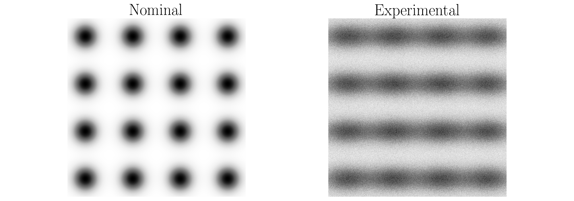
An example use of this function is provided below. The example generates synthetic surfaces representing the nominal and experimental textures. These generated surfaces are shown below where there are 16 features in each image generated using 2D Gaussian distributions similarily to the depth example above. However, for the experimental image in this case, all of the features are elliptical and the additive noise was increased to alter the roundness of the features.
Example:
from scipy.stats import multivariate_normal
import numpy as np
from teaspoon.SP.texture_analysis import feature_roundness

# Generate a grid of sample xy pairs
n = 500
x = np.linspace(-1, 1, n)
y = np.linspace(-1, 1, n)
xv, yv = np.meshgrid(x, y)
xv = xv.reshape(-1, 1)
yv = yv.reshape(-1, 1)
xy = np.column_stack((xv, yv))
nom = 0
exp = 0
ind = 0

# Generate Grid of Strike Locations
grid_size = 4
xc = np.linspace(-0.8, 0.8, grid_size)
yc = np.linspace(-0.8, 0.8, grid_size)
xvc, yvc = np.meshgrid(xc, yc)
xvc = xvc.reshape(-1, 1)
yvc = yvc.reshape(-1, 1)
xyc = np.column_stack((xvc, yvc))


# Generate 3D surface from gaussian distribution and scale between 0-1
for point in xyc:
    ind += 1
    nom += multivariate_normal.pdf(xy, mean=np.array([point[0], point[1]]), cov=np.diag(np.array([0.1, 0.1]) ** 2))
    exp += multivariate_normal.pdf(xy, mean=np.array([point[0], point[1]]), cov=np.diag(np.array([0.2, 0.1]) ** 2))

nom = nom.reshape(n, n).astype(np.float64)
nom = -1.0 * nom + np.max(nom)
nom = nom / np.max(nom) # scale between 0-1

exp = exp.reshape(n, n).astype(np.float64)
exp = -1.0 * exp + np.max(exp)
exp = exp / np.max(exp) # scale between 0-1


# Generate nominal and experimental images by adding noise and scaling from 0-1 again
np.random.seed(48824)
nom_im = nom
exp_im = exp + np.random.normal(scale=0.1, size=[n,n])
exp_im = (exp_im - np.min(exp_im))/(np.max(exp_im) - np.min(exp_im)) # Scale between 0-1

# Compute the roundness score
score = feature_roundness(nom_im, exp_im, 1, 2.5, num_steps=50, plot=True)
Output of example:
roundness_score = 0.11883556
