2.4.1. Time Series Analysis (TSA) Tools

The following are the available TSA functions:

Takens’ Embedding
Permutation Sequence Generation
k Nearest Neighbors
Coarse grained state space binning
Coarse grained state space state sequence
Zero Detection Algorithm (ZeDA)
First Zero Detection Algorithm

Further detailed documentation and examples are provided below for each (or click link).

2.4.1.1. Takens’ Embedding

The Takens’ embedding algorhtm reconstructs the state space from a single time series with delay-coordinate embedding as shown in the animation below.

Figure: Takens’ embedding animation for a simple time series and embedding of dimension two. This embeds the 1-D signal into n=2 dimensions with delayed coordinates.

teaspoon.SP.tsa_tools.takens(ts, n=None, tau=None)[source]

This function generates an array of n-dimensional arrays from a time-delay state-space reconstruction.

Parameters:

ts (1-D array) – 1-D time series signal
n (Optional[int]) – embedding dimension for state space reconstruction. Default is uses FNN algorithm from parameter_selection module.
tau (Optional[int]) – embedding delay fro state space reconstruction. Default uses MI algorithm from parameter_selection module.

Returns:

array of delyed embedded vectors of dimension n for state space reconstruction.

Return type:

[arraay of n-dimensional arrays]

The two parameters needed for state space reconstruction (Takens’ embedding) are the delay parameter and dimension parameter. These can be selected automatically from the parameter selection module ( Parameter selection module documentation).

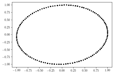
Example:

import numpy as np
t = np.linspace(0,30,200)
ts = np.sin(t)  #generate a simple time series

from teaspoon.SP.tsa_tools import takens
embedded_ts = takens(ts, n = 2, tau = 10)

import matplotlib.pyplot as plt
plt.plot(embedded_ts.T[0], embedded_ts.T[1], 'k.')
plt. show()

Output of example:

2.4.1.2. Permutation Sequence Generation

The function provides an array of the permutations found throughout the time series as shown in the

_images/permutation_sequence_animation.gif

Figure: Permutation sequence animation for a simple time series and permutations of dimension three.

teaspoon.SP.tsa_tools.permutation_sequence(ts, n=None, tau=None)[source]

This function generates the sequence of permutations from a 1-D time series.

Parameters:

ts (1-D array) – 1-D time series signal
n (Optional[int]) – embedding dimension for state space reconstruction. Default is uses MsPE algorithm from parameter_selection module.
tau (Optional[int]) – embedding delay fro state space reconstruction. Default uses MsPE algorithm from parameter_selection module.

Returns:

array of permutations represented as int from [0, n!-1] from the time series.

Return type:

[1-D array of intsegers]

The two parameters needed for permutations are the delay parameter and dimension parameter. These can be selected automatically from the parameter selection module ( Parameter selection module documentation).

Example:

import numpy as np
t = np.linspace(0,30,200)
ts = np.sin(t)  #generate a simple time series

from teaspoon.SP.tsa_tools import permutation_sequence
PS = permutation_sequence(ts, n = 3, tau = 12)

import matplotlib.pyplot as plt
plt.plot(t[:len(PS)], PS, 'k')
plt. show()

Output of example:

2.4.1.3. k Nearest Neighbors

teaspoon.SP.tsa_tools.k_NN(embedded_time_series, k=4)[source]

This function gets the k nearest neighbors from an array of the state space reconstruction vectors

Parameters:

embedded_time_series (array of n-dimensional arrays) – state space reconstructions vectors of dimension n. Can use takens function.
k (Optional[int]) – number of nearest neighbors for graph formation. Default is 4.

Returns:

distances and indices of the k nearest neighbors for each vector.

Return type:

[distances, indices]

Example:

import numpy as np
t = np.linspace(0,15,100)
ts = np.sin(t)  #generate a simple time series

from teaspoon.SP.tsa_tools import takens
embedded_ts = takens(ts, n = 2, tau = 10)

from teaspoon.SP.tsa_tools import k_NN
distances, indices = k_NN(embedded_ts, k=4)


import matplotlib.pyplot as plt
plt.plot(embedded_ts.T[0], embedded_ts.T[1], 'k.')
i = 20 #choose arbitrary index to get NN of.
NN = indices[i][1:] #get nearest neighbors of point with that index.
plt.plot(embedded_ts.T[0][NN], embedded_ts.T[1][NN], 'rs') #plot NN
plt.plot(embedded_ts.T[0][i], embedded_ts.T[1][i], 'bd') #plot point of interest
plt. show()

Output of example:

2.4.1.4. Coarse grained state space binning

Please reference publication “Persistent Homology of the Coarse Grained State Space Network” for details.

teaspoon.SP.tsa_tools.cgss_binning(ts, n=None, tau=None, b=12, binning_method='equal_size', plot_binning=False)[source]

This function generates the binning array applied to each dimension when constructing CGSSN.

Parameters:

ts (1-D array) – 1-D time series signal
n (Optional[int]) – embedding dimension for state space reconstruction. Default is uses MsPE algorithm from parameter_selection module.
tau (Optional[int]) – embedding delay from state space reconstruction. Default uses FNN algorithm from parameter_selection module.
b (Optional[int]) – Number of bins per dimension. Default is 12.
plot_binning (Optional[bool]) – Option to display plotting of binning over space occupied by SSR. default is False.
binning_method (Optional[str]) – Either equal_size or equal_probability for creating binning array. Default is equal_size.

Returns:

One-dimensional array of bin edges.

Return type:

[1-D array]

2.4.1.5. Coarse grained state space state sequence

Please reference publication “Persistent Homology of the Coarse Grained State Space Network” for details.

teaspoon.SP.tsa_tools.cgss_sequence(SSR, B_array)[source]

This function generates the sequence of coarse-grained state space states from the state space reconstruction.

Parameters:

SSR (n-D array) – n-dimensional state state space reconstruction using takens function from teaspoon.
B_array (1-D array) – binning array from function cgss_binning or self defined. Array of bin edges applied to each dimension of SSR for CGSS state sequence.

Returns:

array of coarse grained state space states represented as ints.

Return type:

[1-D array of integers]

2.4.1.6. Zero Detection Algorithm (ZeDA)

This section provides a summary of the zero-crossing detection algorithm devised and analysed in “Robust Zero-crossings Detection in Noisy Signals using Topological Signal Processing” for discrete time series. Additionally, a basic example is provided showing the functionality of the method for a simple time series. Below, a simple overview of the method is provided.

Outline of method: a time series is converted to two point clouds (P) and (Q) based on the sign value. A sorted persistence diagram is generated for both point clouds with x-axis having the index of the data point and y-axis having the death values. Then, a persistence threshold or an outlier detection method is used to select the outlying points in the persistence diagram such that ‘n+1’ points correspond to ‘n’ brackets.

teaspoon.SP.tsa_tools.ZeDA(sig, t1, tn, level=0.0, plotting=False, method='std', score=3.0)[source]

This function takes a uniformly sampled time series and finds level-crossings.

Parameters:

sig (numpy array) – Time series (1d) in format of npy.
t1 (float) – Initial time of recording signal.
tn (float) – Final time of recording signal.
level (Optional[float]) – Level at which crossings are to be found; default: 0.0 for zero-crossings
plotting (Optional[bool]) – Plots the function with returned brackets; defaut is False.
method (Optional[str]) – Method to use for setting persistence threshold; ‘std’ for standard deviation, ‘iso’ for isolation forest, ‘dt’ for smallest time interval in case of a clean signal; default is std (3*standard deviation)
score (Optional[float]) – z-score to use if method == ‘std’; default is 3.0

Returns:

brackets gives intervals in the form of tuples where a crossing is expected; crossings gives the estimated crossings in each interval obtained by averaging both ends; flags marks, for each interval, whether both ends belong to the same sgn(function) category (0, unflagged; 1, flagged)

Return type:

[tuples, list, list]

Example:

import numpy as np
t1 = 0                                          # Initial time value
tn = 1.2                                        # Final time value
t = np.linspace(t1, tn, 200, endpoint=True)     # Generate a time array
sig = (-3*t + 1.4)*np.sin(18*t) + 0.1           # Generate a time series

from teaspoon.SP.tsa_tools import ZeDA

brackets, ZC, flag = ZeDA(sig, t1, tn, plotting=True)

Output of example:

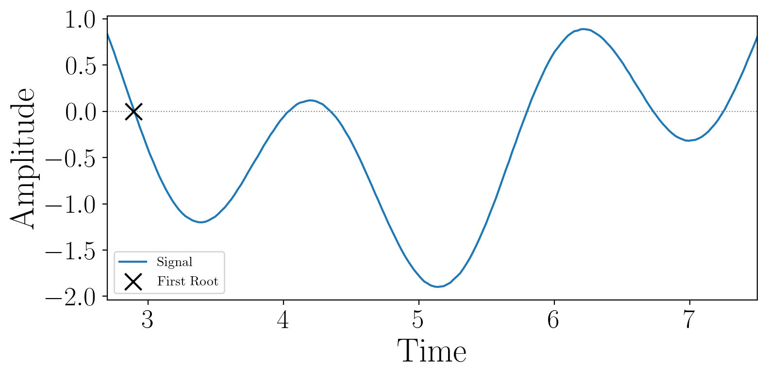
2.4.1.7. First Zero Detection Algorithm

This section provides an implementation of a zero-crossing detection algorithm for the first zero (or the global minimum) in the interval given a discrete time series. This was proposed in “An efficient algorithm for the zero crossing detection in digitized measurement signal”, and was used for benchmarking the algorithm ZeDA above.

teaspoon.SP.tsa_tools.first_zero(sig, t1, tn, level=0.0, r=1.2, plotting=False)[source]

This function takes a discrete time series and finds the first zero-crossing or the global minimum (if no crossing).

Parameters:

sig (numpy array) – Time series (1d) in format of npy.
t1 (float) – Initial time of recording signal.
tn (float) – Final time of recording signal.
level (Optional[float]) – Level at which crossings are to be found; default: 0.0 for zero-crossings
r (Optional[float]) – Reliability (>0)–increasing r increases reliability of the method but may result in a higher convergence time; default: 1.2
plotting (Optional[bool]) – Plots the function with returned brackets; defaut is False.

Returns:

the estimated first crossing in the interval or the global minimum.

Return type:

float

Example:

import numpy as np
t1 = 2.7                                          # Initial time value
tn = 7.5                                        # Final time value
t = np.linspace(t1, tn, 200, endpoint=True)     # Generate a time array
sig = (-3*t + 1.4)*np.sin(18*t) + 0.1           # Generate a time series

from teaspoon.SP.tsa_tools import first_zero

ZC = first_zero(sig, t1, tn, plotting=True)

Output of example: