2.2.2. Featurization
This documentation includes five different persistence diagram featurization methods. These are persistence landscapes, persistence images, Carlsson Coordinates, kernel method, and signature of paths.
2.2.2.1. Persistence Landscapes
2.2.2.1.1. Landscape class
- class teaspoon.ML.feature_functions.PLandscape(PD, L_number=[])[source]
- PLandscape_plot(PL, L_number=[])[source]
This function plots selected persistence landscapes or it plots all of them if user does not provide desired landscape functions.
- Parameters:
PL (ndarray) – Persistence diagram points–(Nx2) matrix.
L_number (list) – Desired landscape numbers in a list form. If the list is empty, all landscapes will be plotted.
- Returns:
PL_plot – The figure that includes chosen or all landsape functions.
- Return type:
figure
- __init__(PD, L_number=[])[source]
This class uses landscapes algorithm (
PD_Featurization.PLandscapes()) to compute persistence landscapes and plot them based on user preference. The algorithm computes the persistence landscapes is written based on Ref. [3].- Parameters:
PD (ndarray) – Persistence diagram points–(Nx2) matrix..
L_number (list) – Desired landscape numbers in a list form. If the list is empty, all landscapes will be plotted.
- Returns:
PL_number (int) – Total number of landscapes for given persistence diagram
DesPL (ndarray) – Includes only selected landscapes functions given in L_number
AllPL (ndarray) – Includes all landscape functions of the persistece diagram
Example: In this example, we do not specify which landscape function we want specifically. Therefore, algorihtms returns a warning to user if desired landscape points is wanted.
>>> from teaspoon.MakeData.PointCloud import testSetManifolds
>>> from teaspoon.ML import feature_functions as Ff
>>> # generate persistence diagrams
>>> df = testSetManifolds(numDgms = 50, numPts = 100)
>>> Diagrams_H1 = df['Dgm1']
>>> # Compute the persistence landscapes
>>> PLC = PLandscape(Diagrams_H1[0])
>>> print(PLC.PL_number)
15
>>> print(PLC.AllPL)
        Landscape Number                                             Points
0                1.0  [[0.5428633093833923, 0.0], [0.580724596977233...
1                2.0  [[0.571907639503479, 0.0], [0.5952467620372772...
2                3.0  [[0.9977497458457947, 0.0], [1.132654219865799...
3                4.0  [[0.9980520009994507, 0.0], [1.132805347442627...
4                5.0  [[1.0069313049316406, 0.0], [1.137244999408722...
5                6.0  [[1.01357901096344, 0.0], [1.0538994073867798,...
6                7.0  [[1.078373670578003, 0.0], [1.0862967371940613...
7                8.0  [[1.1089069843292236, 0.0], [1.188232839107513...
8                9.0  [[1.114268183708191, 0.0], [1.1280720233917236...
9               10.0  [[1.1168304681777954, 0.0], [1.129353165626525...
10              11.0  [[1.1619293689727783, 0.0], [1.214744031429290...
11              12.0  [[1.1846998929977417, 0.0], [1.226129293441772...
12              13.0  [[1.2282723188400269, 0.0], [1.247915506362915...
13              14.0  [[1.2527109384536743, 0.0], [1.260134816169738...
14              15.0  [[1.2588499784469604, 0.0], [1.263204336166381...
>>> print(PLC.DesPL)
Warning: Desired landscape numbers were not specified.
>>> fig = PLC.PLandscape_plot(PLC.AllPL['Points'])
Output of the plotting functions is:
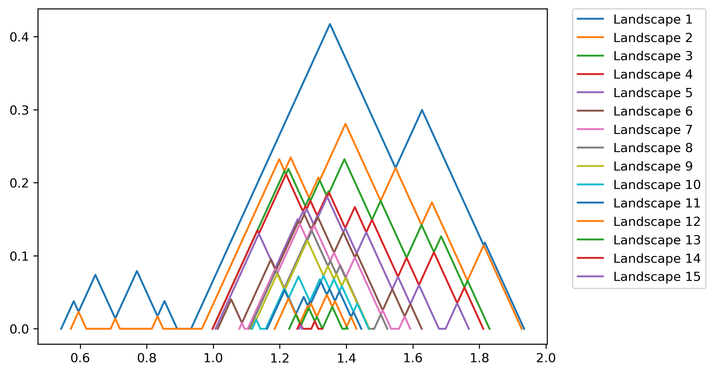
Fig. 2.1 All landscape functions for the given persistence diagram
If user specify the desired landscapes, output will be:
>>> PLC  = PLandscape(Diagrams_H1[0],[2,3])
>>> print(PLC.DesPL)
[array([[0.57190764, 0.        ],
                [0.59524676, 0.02333912],
                [0.61858588, 0.        ],
                [0.69152009, 0.        ],
                [0.70559016, 0.01407006],
                [0.71966022, 0.        ],
                [0.8154344 , 0.        ],
                [0.83258173, 0.01714733],
                [0.84972906, 0.        ],
                [0.96607411, 0.        ],
                [1.19829136, 0.23221725],
                [1.21428031, 0.21622831],
                [1.23277295, 0.23472095],
                [1.28820044, 0.17929345],
                [1.31611174, 0.20720476],
                [1.32007349, 0.20324302],
                [1.39760172, 0.28077126],
                [1.50310916, 0.17526382],
                [1.54805887, 0.22021353],
                [1.62611502, 0.14215738],
                [1.65717965, 0.17322201],
                [1.76435941, 0.06604224],
                [1.81276023, 0.11444306],
                [1.9272033 , 0.        ]])
array([[0.99774975, 0.        ],
                [1.13265422, 0.13490447],
                [1.13280535, 0.13475335],
                [1.21428031, 0.21622831],
                [1.21871996, 0.21178865],
                [1.22592431, 0.21899301],
                [1.27691215, 0.16800517],
                [1.28820044, 0.17929345],
                [1.29216218, 0.17533171],
                [1.32007349, 0.20324302],
                [1.34069568, 0.18262082],
                [1.34636515, 0.1882903 ],
                [1.34829241, 0.18636304],
                [1.3942554 , 0.23232603],
                [1.47721338, 0.14936805],
                [1.50310916, 0.17526382],
                [1.58116531, 0.09720767],
                [1.62611502, 0.14215738],
                [1.66337371, 0.10489869],
                [1.68506891, 0.12659389],
                [1.75498998, 0.05667281],
                [1.76435941, 0.06604224],
                [1.83040166, 0.        ]])]
>>> fig = PLC.PLandscape_plot(PLC.AllPL['Points'],[2,3])
Output of the plotting functions is:
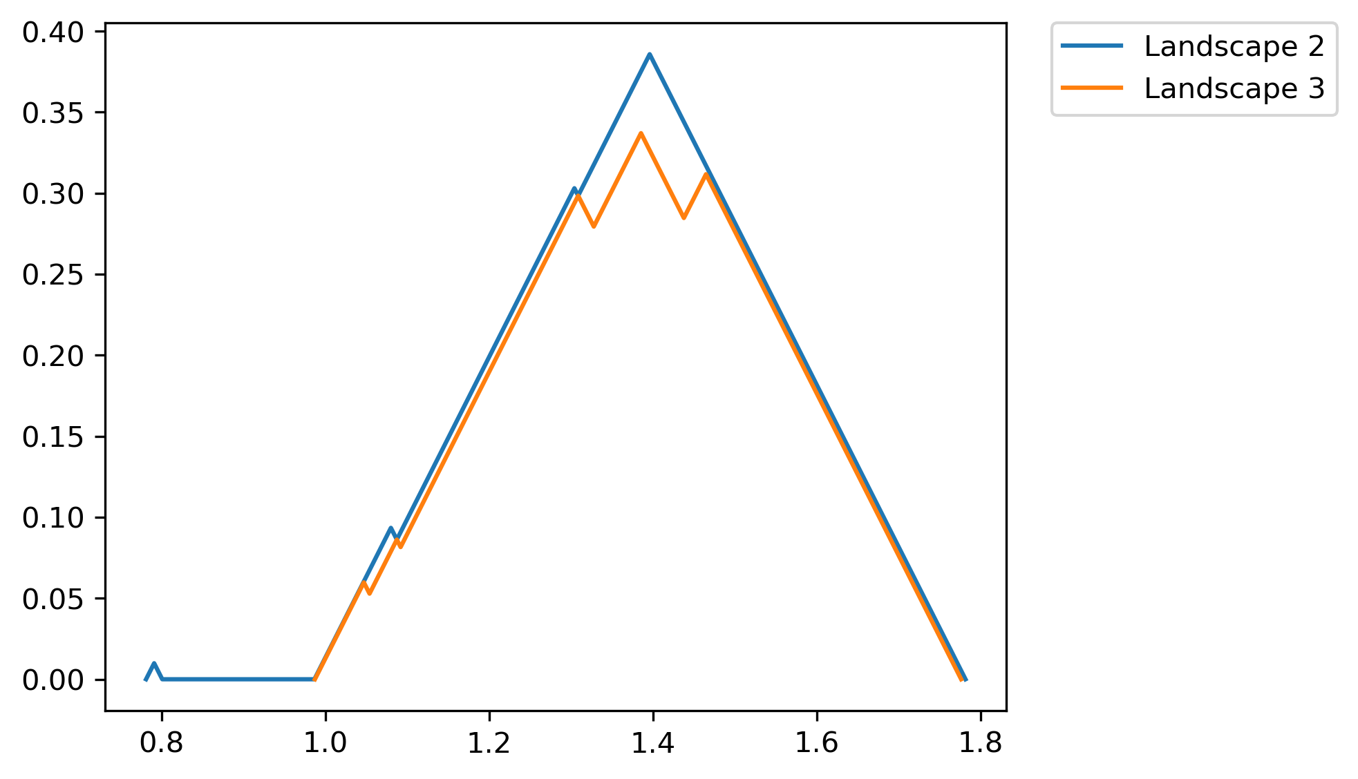
Fig. 2.2 Chosen landscape functions for the given persistence diagram
2.2.2.1.2. Feature matrix generation
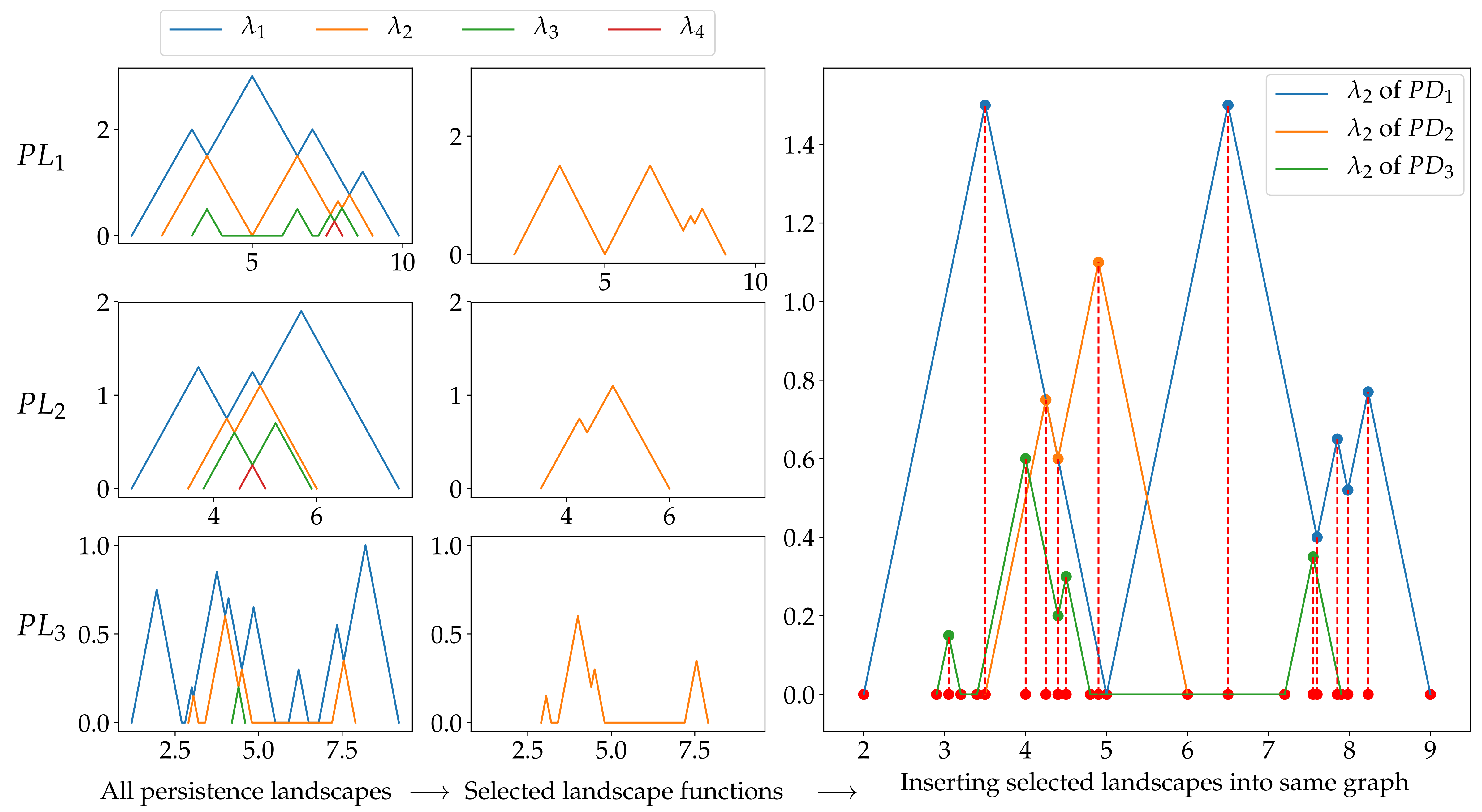
Fig. 2.3 Feature matrix generation steps explained with an simple example.
Fig. 2.3 explains the steps for generation feature matrix using persistence landscapes. There are three persistence landscape sets for three different persistence diagram. We choose one landscape function among them. In the example above, second landscape function is selected and plotted for each landscape set. The plot in the third column includes all selected landscape functions. In other words, we plot all selected landscapes in same figure. The next step is to find the mesh points using node points of landscapes. Node points are projected on x-axis. The red dots in the plot represent these projections. Then, we sort these points (red dots) and remove the duplicates if there is any. Resulting array will be our mesh and it is used to obtain features. The mesh points is shown in Fig. 2.4 with red dots. There may not be corresponding y value for each mesh points in selected landscape functions so we use linear interpolation to find these values. Then, these y values become the feature for each landscape functions, and they can be used in classification.
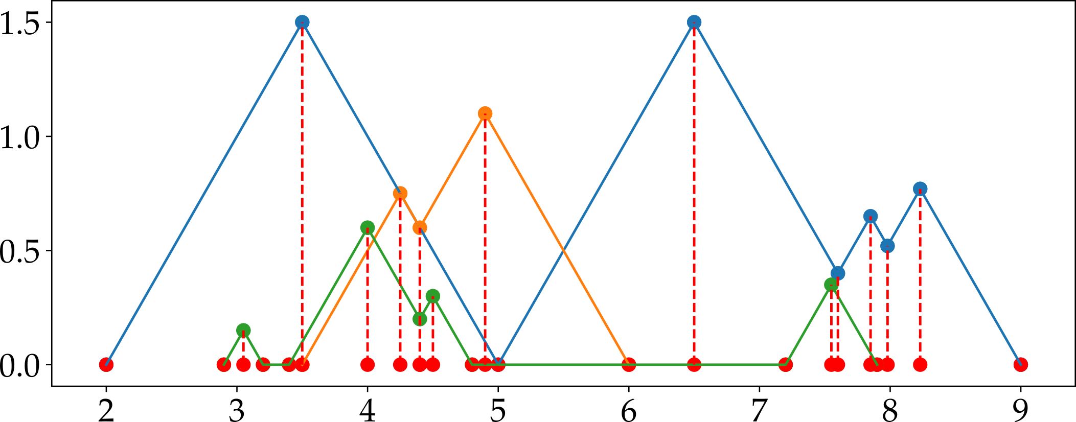
Fig. 2.4 Mesh obtained using second landscape function for the example provided in Fig. 2.3.
- teaspoon.ML.feature_functions.F_Landscape(PL, params, max_l_number=None)[source]
This function computes the features for selected persistence landscape numbers. There are three inputs to the function. These are all landscape functions for each persistence diagram, parameter bucket object and the maximum level of landscape function. If user does not specify the third input, algorithm will automatically compute it. The second parameter includes the parameters needed to compute features and perform classification. Please see
PD_ParameterBucket.LandscapesParameterBucket()for more details about parameters.- Parameters:
PL (ndarray) – Object array that includes all landscape functions for each persistence diagram.
params (parameterbucket object) – Parameterbucket object. We need landscape numbers defined by user to generate feature matrix.
max_l_number (int, optional) – Maximum number of landscape functions for a given persistence diagram. The default is None.
- Returns:
feature (ndarray) – NxM matrix that includes the features for each persistence diagram, where N is the number of persistence diagrams and M is the numbers of features which is equal to length of sorted mesh of landscapes functions.
Sorted_mesh (list) – It includes the sorted mesh for each landscape function chosen by user..
2.2.2.2. Persistence Images
- teaspoon.ML.feature_functions.F_Image(PD1, PS, var, pers_imager=None, training=True, parallel=False)[source]
This function computes the persistence images of given persistence diagrams using Persim package of Python. Then it provides user with the feature matrix for the diagrams.
- Parameters:
PD1 (ndarray) – Object array that includes all persistence diagrams.
PS (float) – Pixel size.
var (float) – Variance of the Gaussian distribution.
pers_imager (persistence image object, optional) – Persistence image object fit to training set diagrams. This oject is only required when the feature function for test set is computed. The default is None.
training (boolean) – This flag tells function if user wants to compute the feature matrix for training and or test set. The default is None.
parallel (boolean) – This flag tells function if user wants to run the computation in parallel. Default is false.
- Returns:
output – Includes feature matrix, persistence image object and persistence images created (for plotting)
- Return type:
dict
Example:
>>> from teaspoon.MakeData.PointCloud import testSetManifolds
>>> from teaspoon.ML import feature_functions as Ff

>>> # generate persistence diagrams
>>> df = testSetManifolds(numDgms=50, numPts=100)
>>> Diagrams_H1 = df['Dgm1'].sort_index().values
>>> PS = 0.01
>>> var = 0.01
>>> feature_PI = Ff.F_Image(Diagrams_H1, PS, var, pers_imager = None,training=True, parallel=True)

>>> # plot example images
>>> Ff.plot_F_Images(feature_PI, num_plots=4, rows=2, cols=2)
The algorithm will return four images as shown in Fig. 2.5. An example notebook is also available.
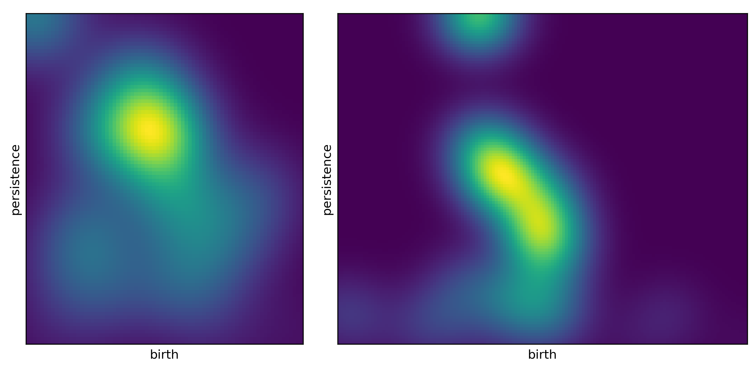
Fig. 2.5 Example persistence images.
2.2.2.3. Carlsson Coordinates
- teaspoon.ML.feature_functions.F_CCoordinates(PD, FN)[source]
This code generates feature matrix to be used in machine learning applications using Carlsson Coordinates which is composed of five different functions shown in Eq. (2.1) - (2.5). The first four functions are taken from Ref. [2] and the last one is obtained from Ref. [6]. There are two inputs to the function. These are persistence diagrams and number of coordinates that user wants to use in feature matrix. Algorithm will return feature matrix object array that includes feature matrices for different combinations, and total number of combinations will be \(\sum_{i=1}^{FN} {FN \choose i}\).
(2.1)\[f_{1}(PD) = \sum b_{i}(d_{i}-b_{i})\](2.2)\[f_{2}(PD) = \sum (d_{max}-d_{i})(d_{i}-b_{i})\](2.3)\[f_{3}(PD) = \sum b_{i}^{2}(d_{i}-b_{i})^{4}\](2.4)\[f_{4}(PD) = \sum (d_{max}-d_{i})^{2}(d_{i}-b_{i})^{4}\](2.5)\[f_{5}(PD) = max(d_{i}-b_{i})\]- Parameters:
PD (ndarray) – Object array that includes all persistence diagrams.
FN (int) – Number of features. It can take integer values between 1 and 5.
- Returns:
FeatureMatrix (object array) – Object array that contains the feature matrices of each feature combinations. Each feature matrix has a size of NxFN, where N is the number of persistence diagrams and FN is the number of feature chosen.
TotalNumComb (int) – Number of combinations.
CombList (list) – List of combinations.
Example:
>>> from teaspoon.MakeData.PointCloud import testSetManifolds
>>> from teaspoon.ML import feature_functions as Ff

>>> # generate persistence diagrams
>>> df = testSetManifolds(numDgms=50, numPts=100)
>>> Diagrams_H1 = df['Dgm1'].sort_index().values

>>> # compute feature matrix
>>> FN = 3
>>> FeatureMatrix, TotalNumComb, CombList = Ff.F_CCoordinates(Diagrams_H1, FN)
2.2.2.4. Template Functions
- teaspoon.ML.feature_functions.tent(Dgm, params, dgm_type='BirthDeath')[source]
Applies the tent function to a diagram.
Parameters:
- Dgm:
A persistence diagram, given as a \(K \times 2\) numpy array
- params:
An tents.ParameterBucket object. Really, we need d, delta, and epsilon from that.
- dgm_type:
- This code accepts diagrams either
in (birth, death) coordinates, in which case type = ‘BirthDeath’, or
in (birth, lifetime) = (birth, death-birth) coordinates, in which case type = ‘BirthLifetime’
- Returns:
\(\sum_{x,y \in \text{Dgm}}g_{i,j}(x,y)\) where
\[\bigg| 1- \max\left\{ \left|\frac{x}{\delta} - i\right|, \left|\frac{y-x}{\delta} - j\right|\right\} \bigg|_+]\]where \(| * |_+\) is positive part; equivalently, min of * and 0.
Note
This code does not take care of the maxPower polynomial stuff. The tbuild_G() function does it after all the rows have been calculated.
- teaspoon.ML.feature_functions.interp_polynomial(Dgm, params, dgm_type='BirthDeath')[source]
Extracts the weights on the interpolation mesh using barycentric Lagrange interpolation.
Parameters:
- Dgm:
A persistence diagram, given as a \(K \times 2\) numpy array
- Params:
An tents.ParameterBucket object. Really, we need d, delta, and epsilon from that.
- Dgm_type:
This code accepts diagrams either 1. in (birth, death) coordinates, in which case type = ‘BirthDeath’, or 2. in (birth, lifetime) = (birth, death-birth) coordinates, in which case dgm_type = ‘BirthLifetime’
- Returns:
- interp_weight
A matrix with each entry representiting the weight of an interpolation function on the base mesh. This matrix assumes that on a 2D mesh the functions are ordered row-wise.
Example:
>>> from teaspoon.MakeData.PointCloud import testSetManifolds
>>> from teaspoon.ML import feature_functions as fF
>>> from teaspoon.ML import Base
>>> import numpy as np
>>> import pandas as pd

>>> # generate persistence diagrams
>>> df = testSetManifolds(numDgms=50, numPts=100)
>>> listOfG = []
>>> dgm_col = ['Dgm0', 'Dgm1']
>>> allDgms = pd.concat((df[label] for label in dgm_col))

>>> # parameter bucket to set template function parameters
>>> params = Base.ParameterBucket()
>>> params.feature_function = fF.interp_polynomial
>>> params.k_fold_cv=5
>>> params.d = 20
>>> params.makeAdaptivePartition(allDgms, meshingScheme=None)
>>> params.jacobi_poly = 'cheb1'  # choose the interpolating polynomial

>>> # compute features
>>> for dgmColLabel in dgm_col:
>>>     feature = Base.build_G(df[dgmColLabel], params)
>>>     listOfG.append(feature)
>>> feature = np.concatenate(listOfG, axis=1)
2.2.2.5. Path Signatures
- teaspoon.ML.feature_functions.F_PSignature(PL, L_Number=[])[source]
This function takes the persistence landscape set and returns the feature matrix which is computed using path signatures [4, 5]. Function takes two inputs and these are persistence landcsape set in an object array and the landscape numbers that user wants to compute their signatures.
- Parameters:
PL (ndarray) – Object array that includes all landscape functions for each persistence diagram.
L_Number (list) – Landscape numbers that user wants to use in feature matrix generation. If this parameter is not specified, algorithm will generate feature matrix using first landscapes.
- Returns:
feature_PS – Nx6 matrix that includes the features for each persistence diagram, where N is the number of persistence landscape sets.
- Return type:
ndarray
Example:
>>> from teaspoon.MakeData.PointCloud import testSetManifolds
>>> from teaspoon.ML import feature_functions as fF
>>> import numpy as np


>>> # generate persistence diagrams
>>> df = testSetManifolds(numDgms=1, numPts=100)
>>> Diagrams_H1 = df['Dgm1'].sort_index().values

>>> # compute persistence landscapes
>>> PerLand = np.ndarray(shape=(6), dtype=object)
>>> for i in range(0, 6):
>>>     Land = fF.PLandscape(Diagrams_H1[i])
>>>     PerLand[i] = Land.AllPL

>>> # choose landscape number for which feature matrix will be computed
>>> L_number = [2]
>>> # compute feature matrix
>>> feature_PS = fF.F_PSignature(PerLand, L_number)
2.2.2.6. Kernel Method
- teaspoon.ML.feature_functions.KernelMethod(perDgm1, perDgm2, sigma)[source]
This function computes the kernel for given two persistence diagram based on the formula provided in Ref. [9]. There are three inputs and these are two persistence diagrams and the kernel scale sigma.
- Parameters:
perDgm1 (ndarray) – Object array that includes first persistence diagram set.
perDgm2 (ndarray) – Object array that includes second persistence diagram set.
sigma (float) – Kernel scale.
- Returns:
Kernel – The kernel value for given two persistence diagrams.
- Return type:
float
Example:
>>> from teaspoon.MakeData.PointCloud import testSetManifolds
>>> from teaspoon.ML import feature_functions as fF
>>> # generate persistence diagrams
>>> df = testSetManifolds(numDgms=1, numPts=100)
>>> Diagrams_H1 = df['Dgm1']
>>> # compute kernel between two persistence diagram
>>> sigma = 0.25
>>> kernel = fF.KernelMethod(Diagrams_H1[0], Diagrams_H1[1], sigma)
>>> print(kernel)
1.6310484200361053