2.1.2.5. Periodic Functions

2.1.2.5.1. Main Functions

teaspoon.MakeData.DynSysLib.periodic_functions.sine(omega=6.283185307179586, L=40, fs=50, SampleSize=2000)

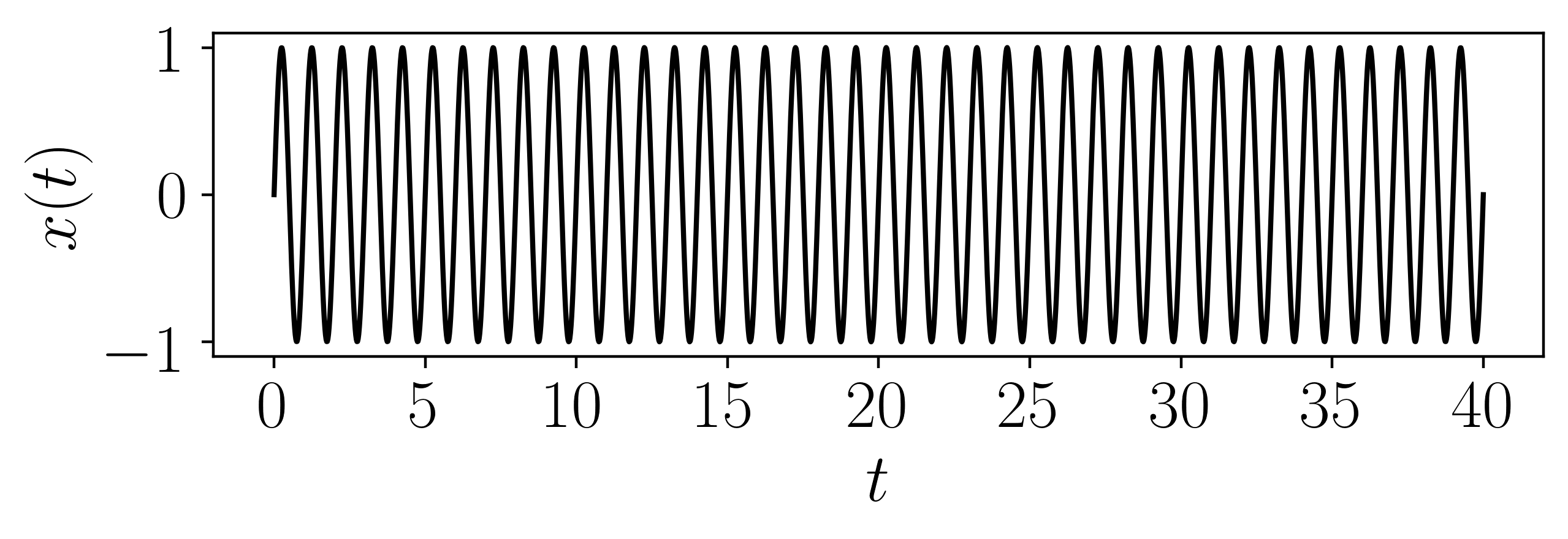
The sinusoidal function is defined as

\[x(t) = \sin(2\pi t)\]

This was solved for 40 seconds with a sampling rate of 50 Hz.

Parameters:

• omega (Optional[float]) – frequency of the sine wave.

• L (Optional[int]) – amount of time to solve simulation for.

• fs (Optional[int]) – sampling rate for simulation.

• SampleSize (Optional[int]) – length of sample at end of entire time series

Returns:

Array of the time indices as t and the simulation time series ts

Return type:

array

teaspoon.MakeData.DynSysLib.periodic_functions.incommensurate_sine(omega1=3.141592653589793, omega2=1, L=100, fs=50, SampleSize=5000)

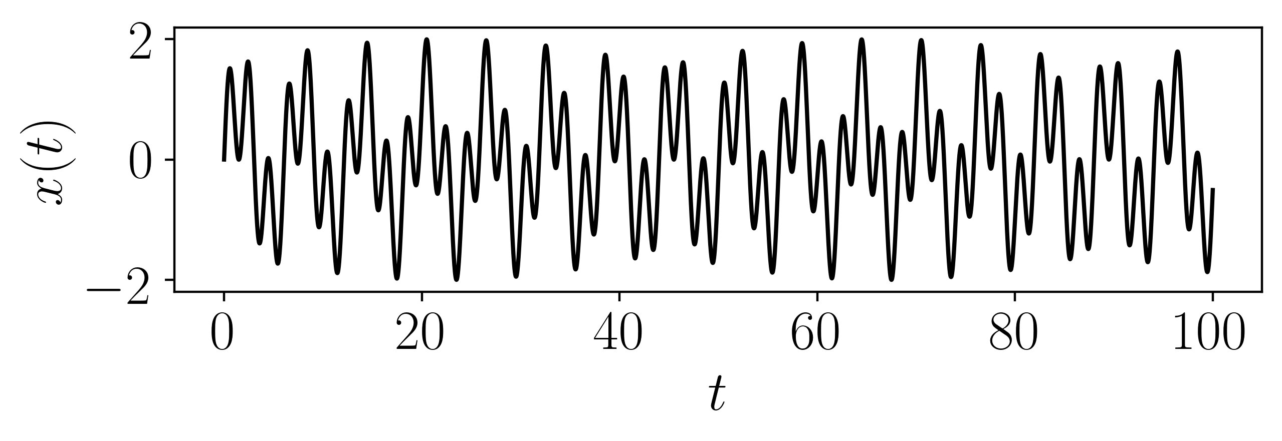
This function is generated using two incommensurate periodic functions as

\[x(t) = \sin(\omega_1 t) + \sin(\omega_2 t)\]

This was sampled such that \(t \in [0, 100]\) at a rate of 50 Hz.

Parameters:

• omega1 (Optional[float]) – frequency of the first sine wave.

• omega2 (Optional[float]) – frequency of the second sine wave.

• L (Optional[int]) – amount of time to solve simulation for.

• fs (Optional[int]) – sampling rate for simulation.

• SampleSize (Optional[int]) – length of sample at end of entire time series

Returns:

Array of the time indices as t and the simulation time series ts

Return type:

array

2.1.2.5.2. Meta Function

This function is for being able to input into the original teaspoon.MakeData.DynSysLib.DynamicSystems function with default parameters.

teaspoon.MakeData.DynSysLib.periodic_functions.periodic_functions(system, dynamic_state=None, L=None, fs=None, SampleSize=None, parameters=None, InitialConditions=None)