2.1.2.4. Conservative Flows

2.1.2.4.1. Main Functions

teaspoon.MakeData.DynSysLib.conservative_flows.simplest_driven_chaotic_flow(fs=50, SampleSize=5000, L=300.0, parameters=[1], InitialConditions=[0, 0], dynamic_state=None)

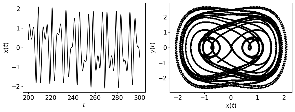
The simplest driven chaotic flow can be reproduced with the following equations

\[ \begin{align}\begin{aligned}\dot{x} = y,\\\dot{y} = -x^3 + \sin{\omega t}\end{aligned}\end{align} \]

where we chose the parameters \((x_0. y_0) = (0.0, 0.0)\) for initial conditions, and \(\omega = 1.0\) (periodic) and \(\omega = 1.88\) (chaotic).

Parameters:

• L (Optional[int]) – Number of iterations.

• fs (Optional[int]) – sampling rate for simulation.

• SampleSize (Optional[int]) – length of sample at end of entire time series

• parameters (Optional[floats]) – array [\(\omega\)] or None if using the dynamic_state variable

• InitialConditions (Optional[floats]) – list of values for [\(x_0\), \(y_0\)]

• dynamic_state (Optional[str]) – Set dynamic state as either ‘periodic’ or ‘chaotic’ if not supplying parameters.

Returns:

Array of the time indices as t and the simulation time series ts

Return type:

array

teaspoon.MakeData.DynSysLib.conservative_flows.nose_hoover_oscillator(fs=20, SampleSize=5000, L=500.0, parameters=[6], InitialConditions=[0, 5, 0], dynamic_state=None)

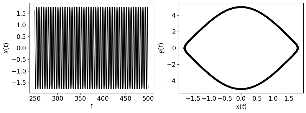
The Nose Hoover Oscillator is represented by the following equations

\[ \begin{align}\begin{aligned}\dot{x} = y,\\\dot{y} = -x + yz,\\\dot{z} = a - y^2\end{aligned}\end{align} \]

where we chose the parameters \((x_0, y_0, z_0) = (0.0, 5.0, 0.0)\) for initial conditions, and \(a = 6.0\) (periodic) and \(a = 1\) (chaotic).

Parameters:

• L (Optional[int]) – Number of iterations.

• fs (Optional[int]) – sampling rate for simulation.

• SampleSize (Optional[int]) – length of sample at end of entire time series

• parameters (Optional[floats]) – list of values for [\(a\)] or None if using the dynamic_state variable

• InitialConditions (Optional[floats]) – list of values for [\(x_0\), \(y_0\), \(z_0\)]

• dynamic_state (Optional[str]) – Set dynamic state as either ‘periodic’ or ‘chaotic’ if not supplying parameters.

Returns:

Array of the time indices as t and the simulation time series ts

Return type:

array

teaspoon.MakeData.DynSysLib.conservative_flows.labyrinth_chaos(fs=10, SampleSize=5000, L=2000.0, parameters=[1, 1, 1], InitialConditions=[0.1, 0, 0], dynamic_state=None)

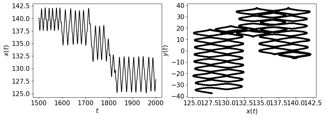
The Labyrinth Chaos Oscillator is represented by the following equations

\[ \begin{align}\begin{aligned}\dot{x} = y,\\\dot{y} = -x + yz,\\\dot{z} = a - y^2\end{aligned}\end{align} \]

where we chose the parameters \((x_0, y_0, z_0) = (0.1, 0.0, 0.0)\) for initial conditions, and \(a = 1.0\) (chaotic) with \(b = 1\) and \(c = 1\). We could not find a periodic response. Any contributions would be appreciated!

Parameters:

• L (Optional[int]) – Number of iterations.

• fs (Optional[int]) – sampling rate for simulation.

• SampleSize (Optional[int]) – length of sample at end of entire time series

• parameters (Optional[floats]) – list of values for [\(a\), \(b\), \(c\)] or None if using the dynamic_state variable

• InitialConditions (Optional[floats]) – list of values for [\(x_0\), \(y_0\), \(z_0\)]

• dynamic_state (Optional[str]) – Set dynamic state as either ‘periodic’ or ‘chaotic’ if not supplying parameters.

Returns:

Array of the time indices as t and the simulation time series ts

Return type:

array

teaspoon.MakeData.DynSysLib.conservative_flows.henon_heiles_system(fs=20, SampleSize=5000, L=10000.0, parameters=[1], InitialConditions=[0.499, 0, 0, 0.03], dynamic_state=None)

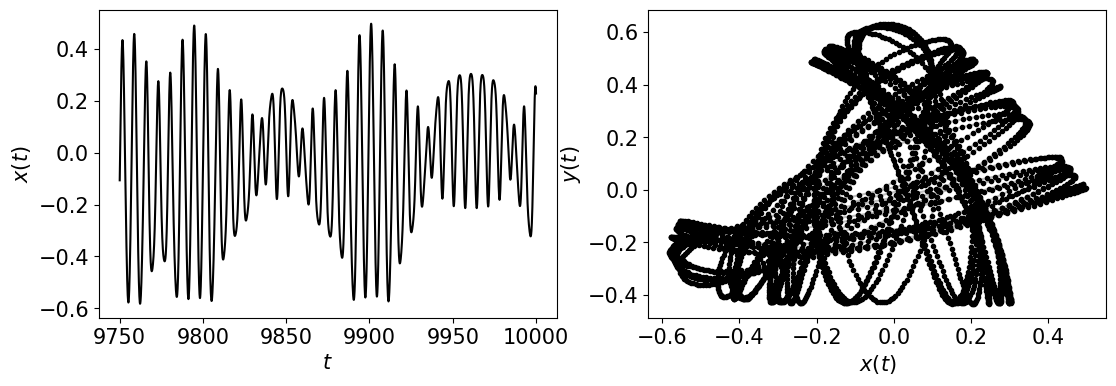
The Henon Heiles System is represented by the following equations

\[ \begin{align}\begin{aligned}\dot{x} = px,\\\dot{px} = -x - 2axy,\\\dot{y} = py,\\\dot{py} = -y - a(x^2 - y^2)\end{aligned}\end{align} \]

where we chose the parameters \((x_0, px_0, y_0, py_0) = (0.499, 0, 0, 0.03)\) for initial conditions, and \(a = 1.0\) (chaotic). We could not find a periodic response. Any contributions would be appreciated!

Parameters:

• L (Optional[int]) – Number of iterations.

• fs (Optional[int]) – sampling rate for simulation.

• SampleSize (Optional[int]) – length of sample at end of entire time series

• parameters (Optional[floats]) – list of values for [\(a\)] or None if using the dynamic_state variable

• InitialConditions (Optional[floats]) – list of values for [\(x_0\), \(px_0\), \(y_0\), \(py_0\)]

• dynamic_state (Optional[str]) – Set dynamic state as either ‘periodic’ or ‘chaotic’ if not supplying parameters.

Returns:

Array of the time indices as t and the simulation time series ts

Return type:

array