2.6.1. Forecasting

This page outlines the available time series forecasting functions.

teaspoon.DAF.forecasting.G_lstm(xp, W_lstm, mu, auto_diff=False)[source]

LSTM Forecast Function with TensorFlow differentiation support.

Parameters:

xp (np.ndarray or tf.Tensor) – Input state vector of shape (D, p)
W_lstm (list) – Model weight arrays to set for the LSTM model (not used here but required for compatibility with other models)
mu (list) – List containing internal model parameters (lstm_units, p, model)
auto_diff (bool) – Enable automatic differentiation functionality

Returns:

Forecasted state vector of shape (D, 1)

Return type:

x_new

teaspoon.DAF.forecasting.G_rfm(xn, W_LR, mu, auto_diff=False)[source]

Random Feature Map Model Forecast Function with TensorFlow differentiation support.

Parameters:

xn (array) – Input state vector (D x 1).
W_LR (array) – Matrix of model coefficients.
mu (list) – List of internal model parameters (W_in, b_in).
auto_diff (bool) – Toggle automatic differentiation for tensorflow usage with TADA.

Returns:

Forecasted state vector (D x 1).

Return type:

x_new (array)

teaspoon.DAF.forecasting.forecast_time(X_model_a, X_truth, dt=1.0, lambda_max=1.0, threshold=0.05)[source]

Function to compute the forecast time using the relative forecast error to compare predictions to measurements with a threshold.

Parameters:

X_model_a (array) – Array of forecast points
X_truth (array) – Array of measurements (ground truth)
dt (float) – Time step size (defaults to 1 to return number of points)
lambda_max (float) – Maximum lyapunov exponent (defaults to 1 to return number of points)
threshold (float) – Threshold to use for comparing forecast and measurements.

Returns:

Forecast time for the given threshold.

Return type:

(float)

teaspoon.DAF.forecasting.get_forecast(Xp, W, mu, forecast_len, G=<function G_rfm>, auto_diff=False)[source]

Function for computing a forecast from a given forecast model.

Parameters:

Xp (array) – Starting point(s) for the forecast (D x p) vector.
W (array/object) – Model weights or model object for making predictions.
mu (list) – List of internal model parameters (model specific).
forecast_len (int) – Number of points to forecast into the future.
G (function) – Forecast function. Defaults to random feature map (G_rfm).
auto_diff (bool) – Toggle automatic differentiation for tensorflow usage with TADA.

Returns:

Array of forecasted states.

Return type:

forecast (array)

teaspoon.DAF.forecasting.lstm_model(u_obs, units=500, p=1, epochs=50, batch_size=50)[source]

Function for generating a LSTM forecast model

Parameters:

u_obs (array) – Array of observations (D x N) D is the dimension, N is the number of training points.
units (int) – Number of LSTM units.
p (int) – Number of past points to use for predicting the next point.
epochs (int) – Number of LSTM training epochs.
batch_size (int) – Training batch size for LSTM model.

Returns:

Trained LSTM model.

Return type:

model (keras Sequential)

teaspoon.DAF.forecasting.random_feature_map_model(u_obs, Dr, w=0.005, b=4.0, beta=4e-05, seed=None)[source]

Function for generating a random feature map dynamical system model based on the method presented in https://doi.org/10.1016/j.physd.2021.132911.

Parameters:

u_obs (array) – Array of observations (D x N) D is the dimension, N is the number of training points.
Dr (int) – Reservoir dimension
w (float) – Random feature weight matrix distribution width parameter.
b (float) – Random feature bias vector distribution parameter.
beta (float) – Ridge regression regularization parameter.
seed (int) – Random seed (optional)

Returns:

Optimal model weights. W_in (array): Random weight matrix. b_in (array): Random bias vector.

Return type:

W_LR (array)

Example:

import numpy as np
from matplotlib import rc
import matplotlib.pyplot as plt
from matplotlib.gridspec import GridSpec
from teaspoon.MakeData.DynSysLib.autonomous_dissipative_flows import lorenz
from teaspoon.DAF.forecasting import random_feature_map_model
from teaspoon.DAF.forecasting import get_forecast


# Set font
rc('font', **{'family': 'sans-serif', 'sans-serif': ['Helvetica']})
rc('text', usetex=True)
plt.rc('text', usetex=True)
plt.rc('font', family='serif')
plt.rcParams.update({'font.size': 16})

# Set model parameters
Dr=300
train_len = 4000
forecast_len = 2000

r_seed = 48824
np.random.seed(r_seed)

# Get training and tesing data at random initial condition
ICs = list(np.random.normal(size=(3,1)).reshape(-1,))
t, ts = lorenz(L=500, fs=50, SampleSize=6001, parameters=[28,10.0,8.0/3.0],InitialConditions=ICs)
ts = np.array(ts)

# Add noise to signals
noise = np.random.normal(scale=0.01, size=np.shape(ts[:,0:train_len+forecast_len]))
u_obs = ts[:,0:train_len+forecast_len] + noise

# Train model
W_LR, W_in, b_in = random_feature_map_model(u_obs[:,0:train_len],Dr, seed=r_seed)

# Generate forecast
forecast_len = 500
X_model= get_forecast(u_obs[:,train_len].reshape(-1,1), W_LR, mu=(W_in, b_in),forecast_len=forecast_len)
X_meas = u_obs[:,train_len:train_len+forecast_len]

# Plot measurements and forecast
fig = plt.figure(figsize=(15, 5))
gs = GridSpec(1, 3)
ax1 = fig.add_subplot(gs[0, 0])
ax1.plot(X_model[0,:],'r', label="Forecast")
ax1.plot(X_meas[0,:], '.b', label="Measurement")
ax1.plot([],[])
ax1.set_title('x', fontsize='x-large')
ax1.tick_params(axis='both', which='major', labelsize='x-large')
ax1.set_ylim((-30,30))


ax2 = fig.add_subplot(gs[0, 1])
ax2.plot(X_model[1,:],'r', label="Forecast")
ax2.plot(X_meas[1,:], '.b', label="Measurement")
ax2.plot([],[])
ax2.set_title('y', fontsize='x-large')
ax2.tick_params(axis='both', which='major', labelsize='x-large')
ax2.set_ylim((-30,30))

ax3 = fig.add_subplot(gs[0, 2])
ax3.plot(X_model[2,:],'r', label="Forecast")
ax3.plot(X_meas[2,:], '.b', label="Measurement")
ax3.plot([],[])
ax3.legend(fontsize='large', loc='upper left')
ax3.set_title('z', fontsize='x-large')
ax3.tick_params(axis='both', which='major', labelsize='x-large')
ax3.set_ylim((0,60))

plt.tight_layout()
plt.show()

Output of example

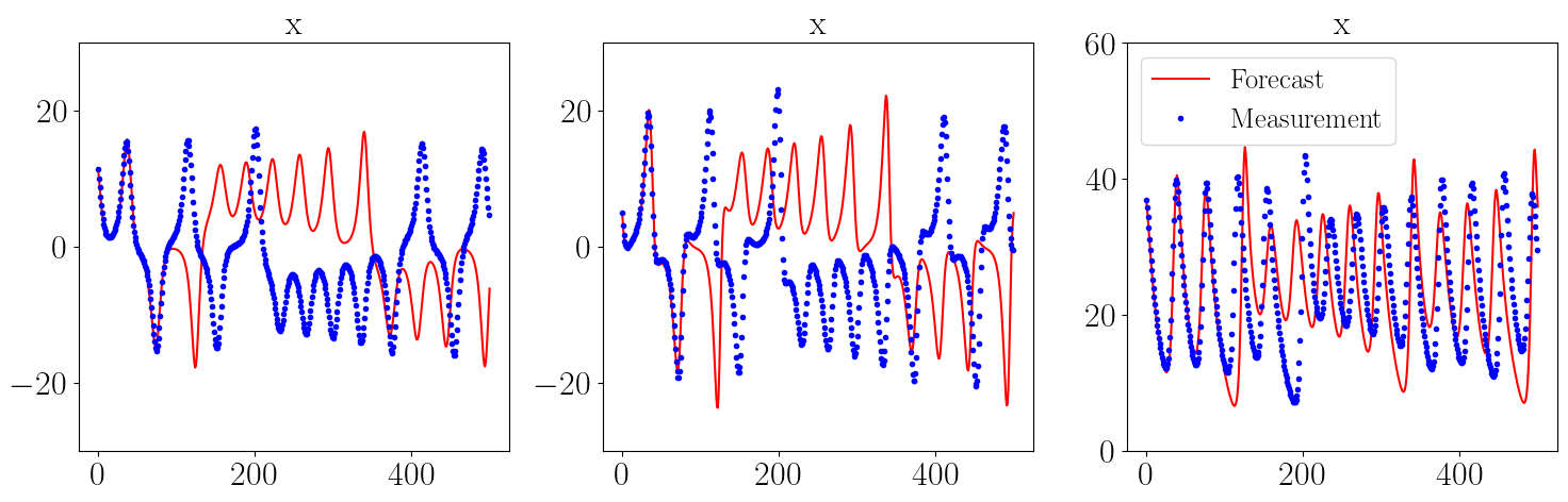
Note

Forecast may vary depending on the operating system.