2.1.2.1. Maps
2.1.2.1.1. Main Functions
- teaspoon.MakeData.DynSysLib.maps.logistic_map(parameters=[3.5], dynamic_state=None, InitialConditions=None, L=1000.0, fs=1, SampleSize=500)[source]
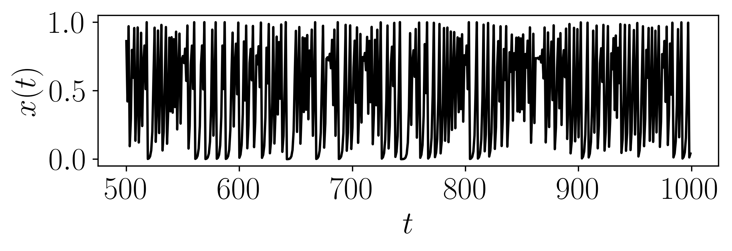
The logistic map [1] was generated as
\[x_{n+1} = rx_n(1-x_n)\]where we chose the parameters \(x_0 = 0.5\) and \(r = 3.6\) for a chaotic state. You can set \(r = 3.5\) for a periodic response. We solve this system for 1000 data points and keep the second 500 to avoid transients.

- Parameters:
parameters (Optional[float]) – Array of 1 float [r]
dynamic_state (Optional[string]) – Dynamic state (‘periodic’ or ‘chaotic’)
L (Optional[int]) – Number of map iterations.
fs (Optional[int]) – sampling rate for simulation.
SampleSize (Optional[int]) – length of sample at end of entire time series
- Returns:
Array of the time indices as t and the simulation time series ts
- Return type:
array
References
- teaspoon.MakeData.DynSysLib.maps.henon_map(parameters=[1.25, 0.3, 1.0], dynamic_state=None, InitialConditions=None, L=1000.0, fs=1, SampleSize=500)[source]
The Hénon map [2] was solved as
\[ \begin{align}\begin{aligned}x_{n+1} &= 1 -ax_n^2+y_n,\\y_{n+1}&=bx_n\end{aligned}\end{align} \]where we chose the parameters \(a = 1.20\), \(b = 0.30\), and \(c = 1.00\) for a chaotic state with initial conditions \(x_0 = 0.1\) and \(y_0 = 0.3\). You can set \(a = 1.25\) for a periodic response. We solve this system for 1000 data points and keep the second 500 to avoid transients.
- Parameters:
parameters (Optional[floats]) – Array of 3 floats [a,b,c].
dynamic_state (Optional[string]) – Dynamic state (‘periodic’ or ‘chaotic’)
L (Optional[int]) – Number of map iterations.
fs (Optional[int]) – sampling rate for simulation.
SampleSize (Optional[int]) – length of sample at end of entire time series
- Returns:
Array of the time indices as t and the simulation time series ts
- Return type:
array
References
- teaspoon.MakeData.DynSysLib.maps.sine_map(parameters=[0.8], dynamic_state=None, InitialConditions=None, L=1000.0, fs=1, SampleSize=500)[source]
The Sine map is defined as
\[x_{n+1} = A\sin{(\pi x_n)}\]where we chose the parameter \(A = 1.0\) for a chaotic state with initial condition \(x_0 = 0.1\). You can also change \(A = 0.8\) for a periodic response. We solve this system for 1000 data points and keep the second 500 to avoid transients.
- Parameters:
parameters (Optional[floats]) – Array of 1 float [A].
dynamic_state (Optional[string]) – Dynamic state (‘periodic’ or ‘chaotic’)
L (Optional[int]) – Number of map iterations.
fs (Optional[int]) – sampling rate for simulation.
SampleSize (Optional[int]) – length of sample at end of entire time series
- Returns:
Array of the time indices as t and the simulation time series ts
- Return type:
array
- teaspoon.MakeData.DynSysLib.maps.tent_map(parameters=[1.05], dynamic_state=None, InitialConditions=None, L=1000.0, fs=1, SampleSize=500)[source]
The Tent map [3] was solved as
\[x_{n+1} = A\min{([x_n, 1-x_n])}\]where we chose the parameter \(A = 1.50\) for a chaotic state with initial condition \(x_0 = 1/\sqrt{2}\). You can also change \(A = 1.05\) for a periodic response. We solve this system for 1000 data points and keep the second 500 to avoid transients.
- Parameters:
parameters (Optional[float]) – Array of 1 float [A].
dynamic_state (Optional[string]) – Dynamic state (‘periodic’ or ‘chaotic’)
L (Optional[int]) – Number of map iterations.
fs (Optional[int]) – sampling rate for simulation.
SampleSize (Optional[int]) – length of sample at end of entire time series
- Returns:
Array of the time indices as t and the simulation time series ts
- Return type:
array
References
- teaspoon.MakeData.DynSysLib.maps.linear_congruential_generator_map(parameters=[0.9, 54773, 259200], dynamic_state=None, InitialConditions=None, L=1000.0, fs=1, SampleSize=500)[source]
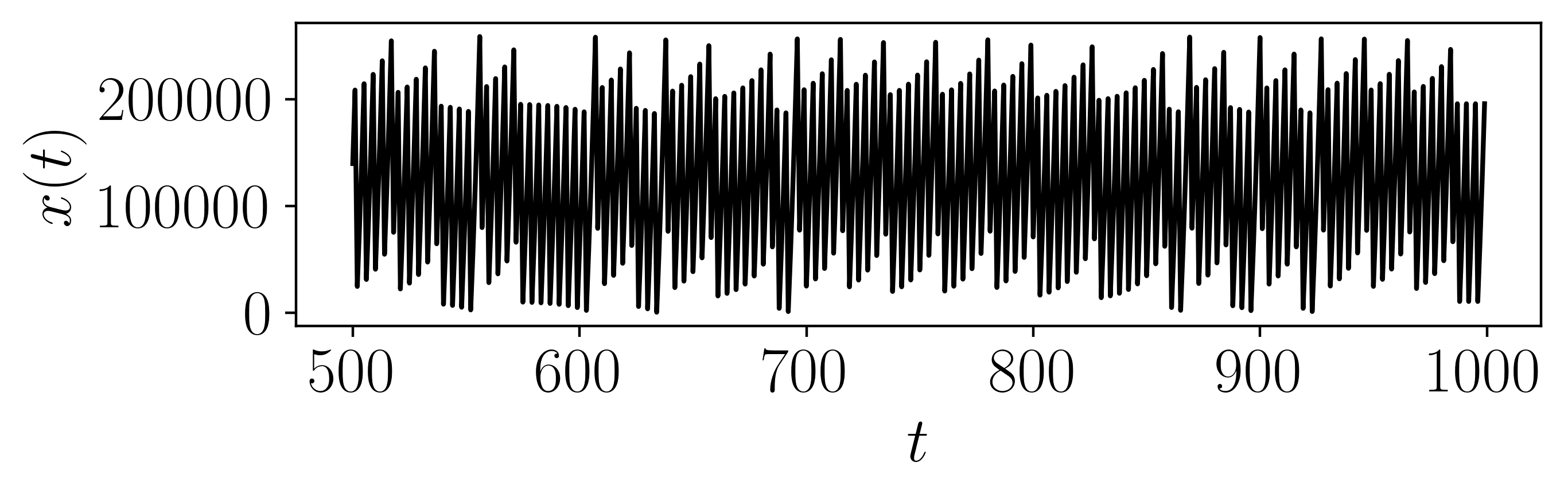
The Linear Congruential Generator map is defined as
\[x_{n+1}=(ax_n+b)\mod c\]where we chose the parameter \(a = 1.1\) for a chaotic state with initial condition \(x_0 = 0.1\). You can also change \(a = 0.9\) for a periodic response. \(b\) and \(c\) are set to 54,773 and 259,200 respectively for both dynamic states. We solve this system for 1000 data points and keep the second 500 to avoid transients.
- Parameters:
parameters (Optional[float]) – Array of 3 floats [a,b,c].
dynamic_state (Optional[string]) – Dynamic state (‘periodic’ or ‘chaotic’)
L (Optional[int]) – Number of map iterations.
fs (Optional[int]) – sampling rate for simulation.
SampleSize (Optional[int]) – length of sample at end of entire time series
- Returns:
Array of the time indices as t and the simulation time series ts
- Return type:
array
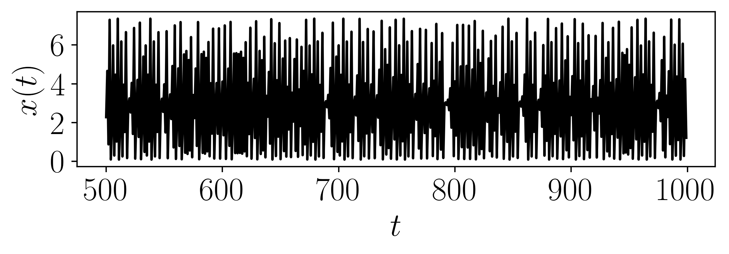
- teaspoon.MakeData.DynSysLib.maps.rickers_population_map(parameters=[13], dynamic_state=None, InitialConditions=None, L=1000.0, fs=1, SampleSize=500)[source]
The Ricker’s Population map is defined [4] as
\[x_{n+1}=ax_n e^{-x_n}\]where we chose the parameter \(a = 20\) for a chaotic state with initial condition \(x_0 = 0.1\). You can set \(a = 13\) for a periodic response. We solve this system for 1000 data points and keep the second 500 to avoid transients.
- Parameters:
parameters (Optional[float]) – Array of 1 parameter [a].
dynamic_state (Optional[string]) – Dynamic state (‘periodic’ or ‘chaotic’)
L (Optional[int]) – Number of map iterations.
fs (Optional[int]) – sampling rate for simulation.
SampleSize (Optional[int]) – length of sample at end of entire time series
- Returns:
Array of the time indices as t and the simulation time series ts
- Return type:
array
References
- teaspoon.MakeData.DynSysLib.maps.gauss_map(parameters=[6.2, -0.2], dynamic_state=None, InitialConditions=None, L=1000.0, fs=1, SampleSize=500)[source]
The Gauss map is defined [5] as
\[x_{n+1}=e^{-\alpha x_n^2}+\beta\]where we chose the parameters \(\alpha = 6.20\) and \(\beta = -0.35\) for a chaotic state with initial condition \(x_0 = 0.1\). You can set \(\beta = -0.20\) for a periodic response. We solve this system for 1000 data points and keep the second 500 to avoid transients. Taken from https://en.wikipedia.org/wiki/Gauss_iterated_map
- Parameters:
parameters (Optional[floats]) – Array of parameters [alpha, beta].
beta (Optional[float]) – System parameter.
dynamic_state (Optional[string]) – Dynamic state (‘periodic’ or ‘chaotic’)
L (Optional[int]) – Number of map iterations.
fs (Optional[int]) – sampling rate for simulation.
SampleSize (Optional[int]) – length of sample at end of entire time series
- Returns:
Array of the time indices as t and the simulation time series ts
- Return type:
array
References
- teaspoon.MakeData.DynSysLib.maps.cusp_map(parameters=[1.1], dynamic_state=None, InitialConditions=None, L=1000.0, fs=1, SampleSize=500)[source]
The Cusp map is defined [6] as
\[x_{n+1} = 1 - a\sqrt{|x_n|}\]where we chose the parameter \(a = 1.2\) for a chaotic state with initial condition \(x_0 = 0.5\). You can set \(a = 1.1\) for a periodic response. We solve this system for 1000 data points and keep the second 500 to avoid transients.
- Parameters:
parameters (Optional[float]) – Array of system parameters [a].
dynamic_state (Optional[string]) – Dynamic state (‘periodic’ or ‘chaotic’)
L (Optional[int]) – Number of map iterations.
fs (Optional[int]) – sampling rate for simulation.
SampleSize (Optional[int]) – length of sample at end of entire time series
- Returns:
Array of the time indices as t and the simulation time series ts
- Return type:
array
References
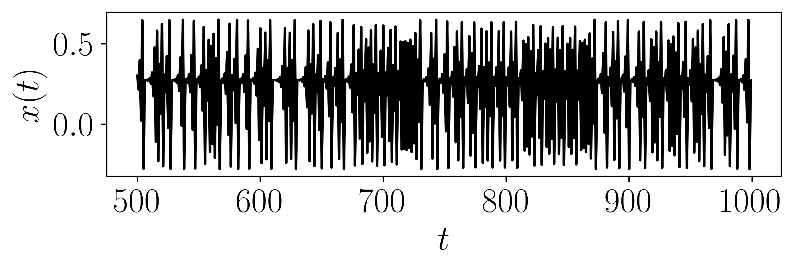
- teaspoon.MakeData.DynSysLib.maps.pinchers_map(parameters=[1.3, 0.5], dynamic_state=None, InitialConditions=None, L=1000.0, fs=1, SampleSize=500)[source]
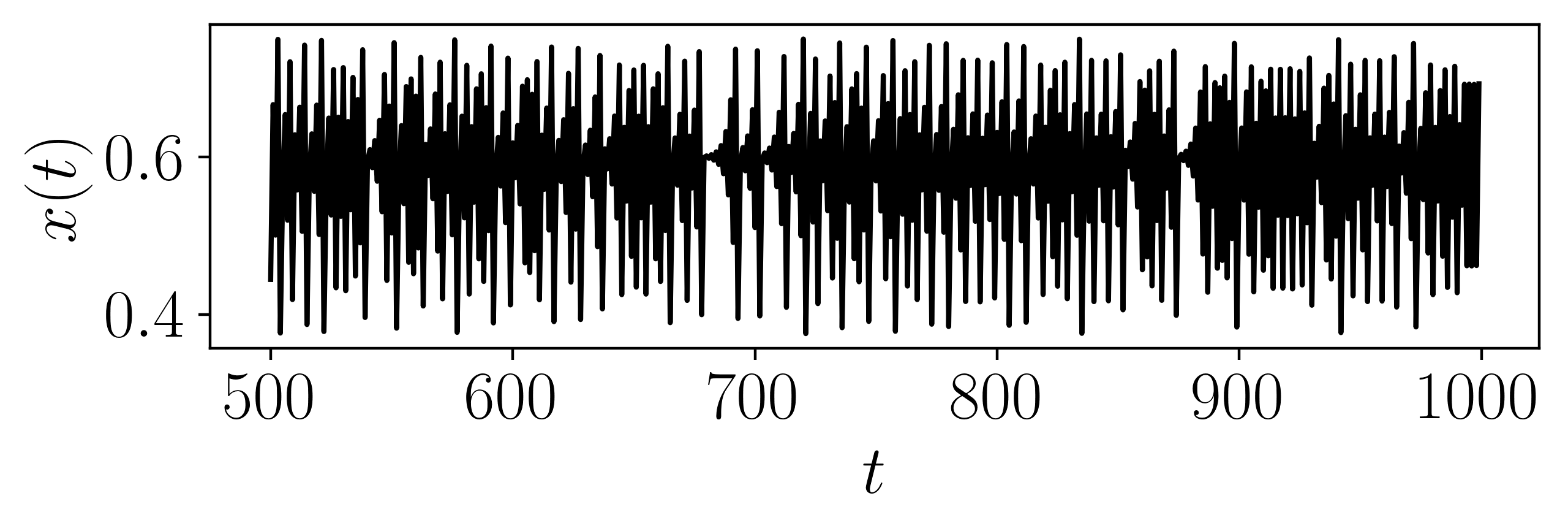
The Pincher’s map is defined [7] as
\[x_{n+1} = |\tanh{(s(x_n-c))}|\]where we chose the parameters \(s = 1.6\) and \(c = 0.5\) for a chaotic state with initial condition \(x_0 = 0.0\). You can set \(s = 1.3\) for a periodic response. We solve this system for 1000 data points and keep the second 500 to avoid transients.

- Parameters:
parameters (Optional[float]) – Array of system parameters [s,c].
dynamic_state (Optional[string]) – Dynamic state (‘periodic’ or ‘chaotic’)
L (Optional[int]) – Number of map iterations.
fs (Optional[int]) – sampling rate for simulation.
SampleSize (Optional[int]) – length of sample at end of entire time series
- Returns:
Array of the time indices as t and the simulation time series ts
- Return type:
array
References
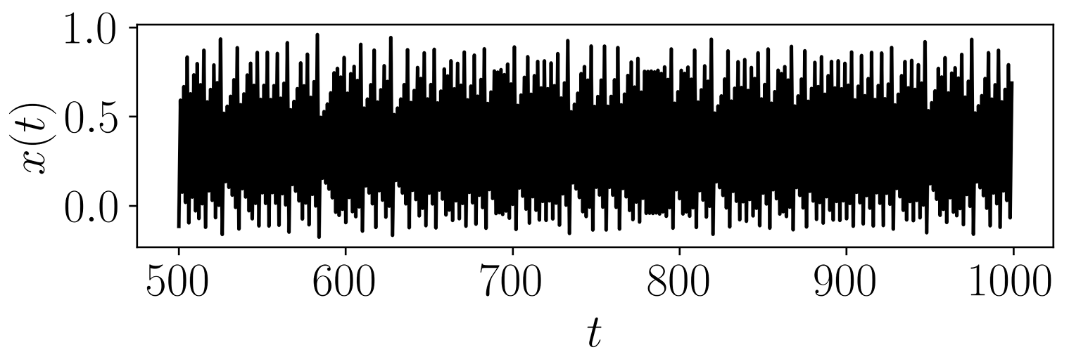
- teaspoon.MakeData.DynSysLib.maps.sine_circle_map(parameters=[0.5, 1.5], dynamic_state=None, InitialConditions=None, L=1000.0, fs=1, SampleSize=500)[source]
The Sine Circle map is defined [8] as
\[x_{n+1} = x_n + \omega -\left[\frac{k}{2\pi}\sin{(2\pi x_n)}\right]\]where we chose the parameters \(\omega = 0.5\) and \(k = 2.0\) for a chaotic state with initial condition \(x_0 = 0.0\). You can set \(k = 1.5\) for a periodic response. We solve this system for 1000 data points and keep the second 500 to avoid transients.
- Parameters:
parameters (Optional[float]) – Array of system parameters [omega, k].
dynamic_state (Optional[string]) – Dynamic state (‘periodic’ or ‘chaotic’)
L (Optional[int]) – Number of map iterations.
fs (Optional[int]) – sampling rate for simulation.
SampleSize (Optional[int]) – length of sample at end of entire time series
- Returns:
Array of the time indices as t and the simulation time series ts
- Return type:
array
References
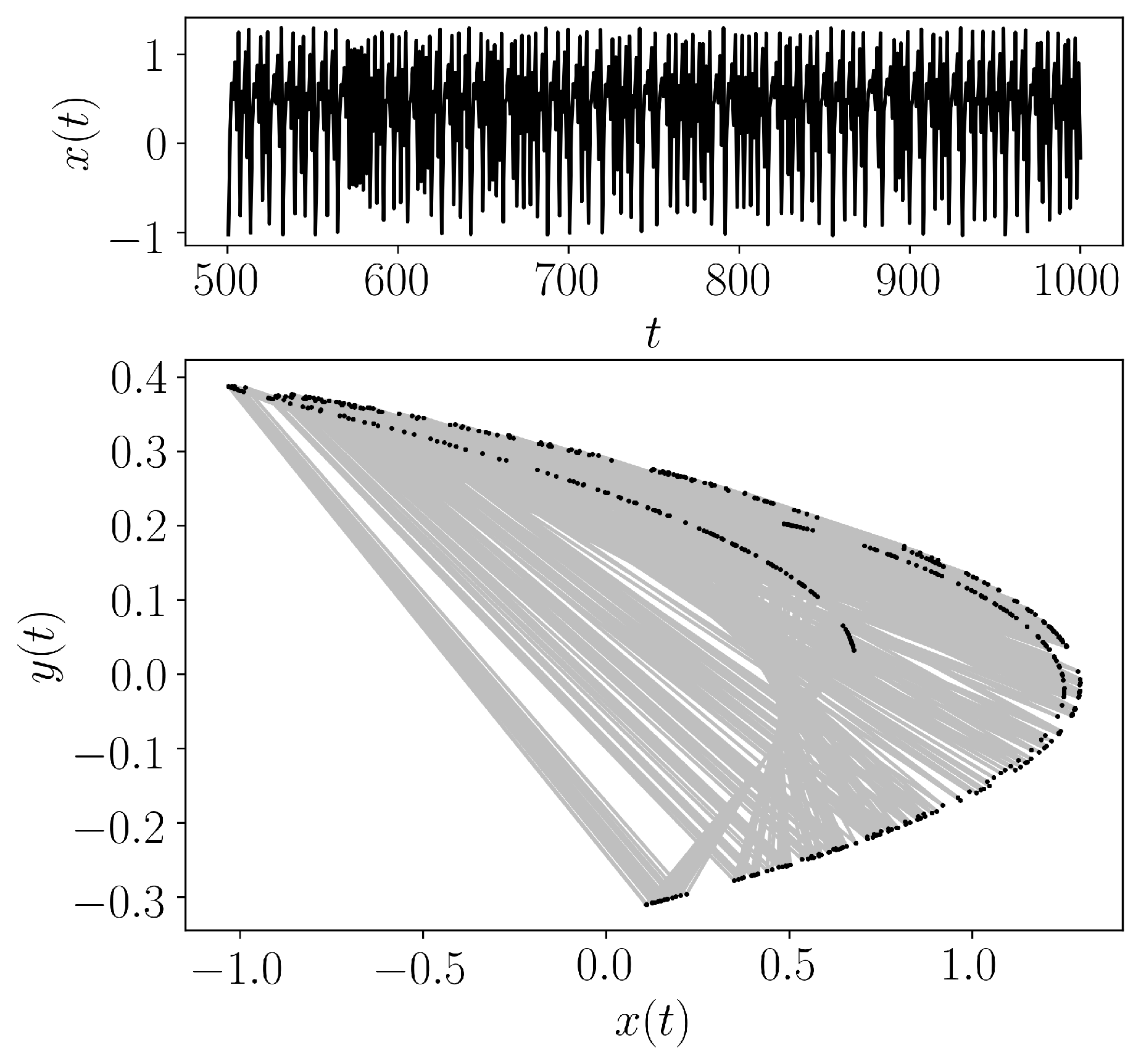
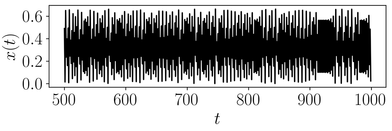
- teaspoon.MakeData.DynSysLib.maps.lozi_map(parameters=[1.5, 0.5], dynamic_state=None, InitialConditions=None, L=1000.0, fs=1, SampleSize=500)[source]
The Lozi map is defined [9] as
\[ \begin{align}\begin{aligned}x_{n+1} &= 1 - a|x_n| +by_n,\\y_{n+1} &= x_n\end{aligned}\end{align} \]where we chose the parameters \(a = 1.7\) and \(b = 0.5\) for a chaotic state with initial conditions \(x_0 = -0.1\) and \(y_0 = 0.1\). You can set \(a = 1.5\) for a periodic response. We solve this system for 1000 data points and keep the second 500 to avoid transients.
- Parameters:
parameters (Optional[float]) – Array of system parameters [a,b].
dynamic_state (Optional[string]) – Dynamic state (‘periodic’ or ‘chaotic’)
L (Optional[int]) – Number of map iterations.
fs (Optional[int]) – sampling rate for simulation.
SampleSize (Optional[int]) – length of sample at end of entire time series
- Returns:
Array of the time indices as t and the simulation time series ts
- Return type:
array
References
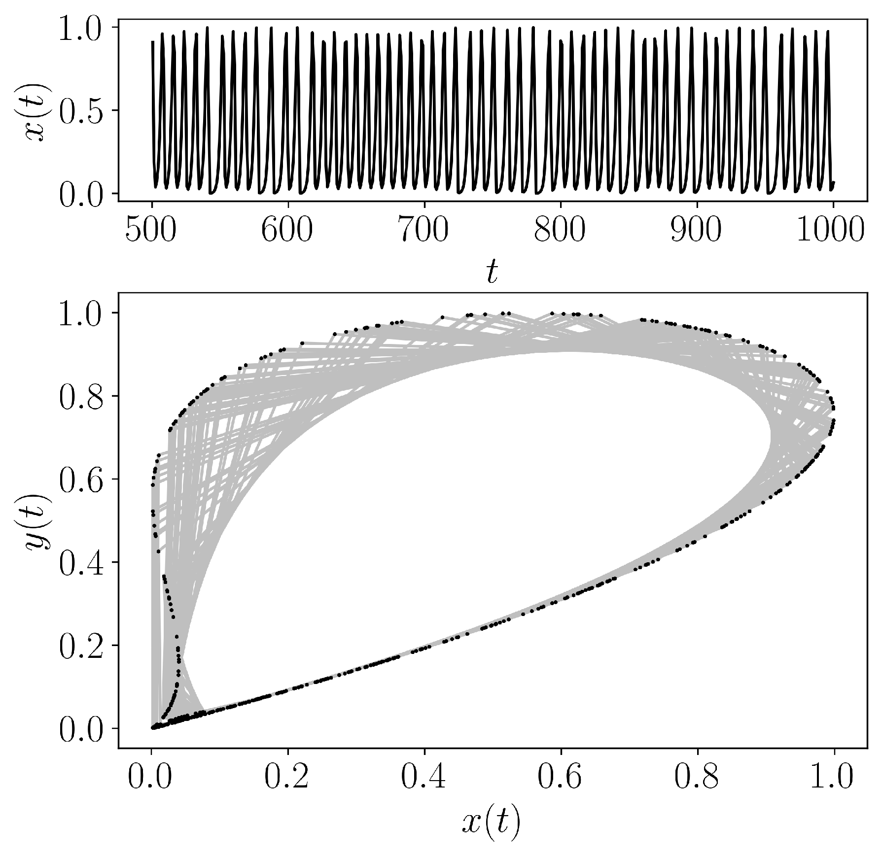
- teaspoon.MakeData.DynSysLib.maps.delayed_logstic_map(parameters=[2.2], dynamic_state=None, InitialConditions=None, L=1000.0, fs=1, SampleSize=500)[source]
The Delayed Logistic map is defined [10] as
\[ \begin{align}\begin{aligned}x_{n+1} &= ax_n(1-y_n)\\y_{n+1} &= x_n\end{aligned}\end{align} \]where we chose the parameter \(a = 2.27\) for a chaotic state with initial conditions \(x_0 = 0.001\) and \(y_0 = 0.001\). You can set \(a = 2.20\) for a periodic response. We solve this system for 1000 data points and keep the second 500 to avoid transients.
- Parameters:
parameters (Optional[float]) – Array of system parameters [a].
dynamic_state (Optional[string]) – Dynamic state (‘periodic’ or ‘chaotic’)
L (Optional[int]) – Number of map iterations.
fs (Optional[int]) – sampling rate for simulation.
SampleSize (Optional[int]) – length of sample at end of entire time series
- Returns:
Array of the time indices as t and the simulation time series ts
- Return type:
array
References
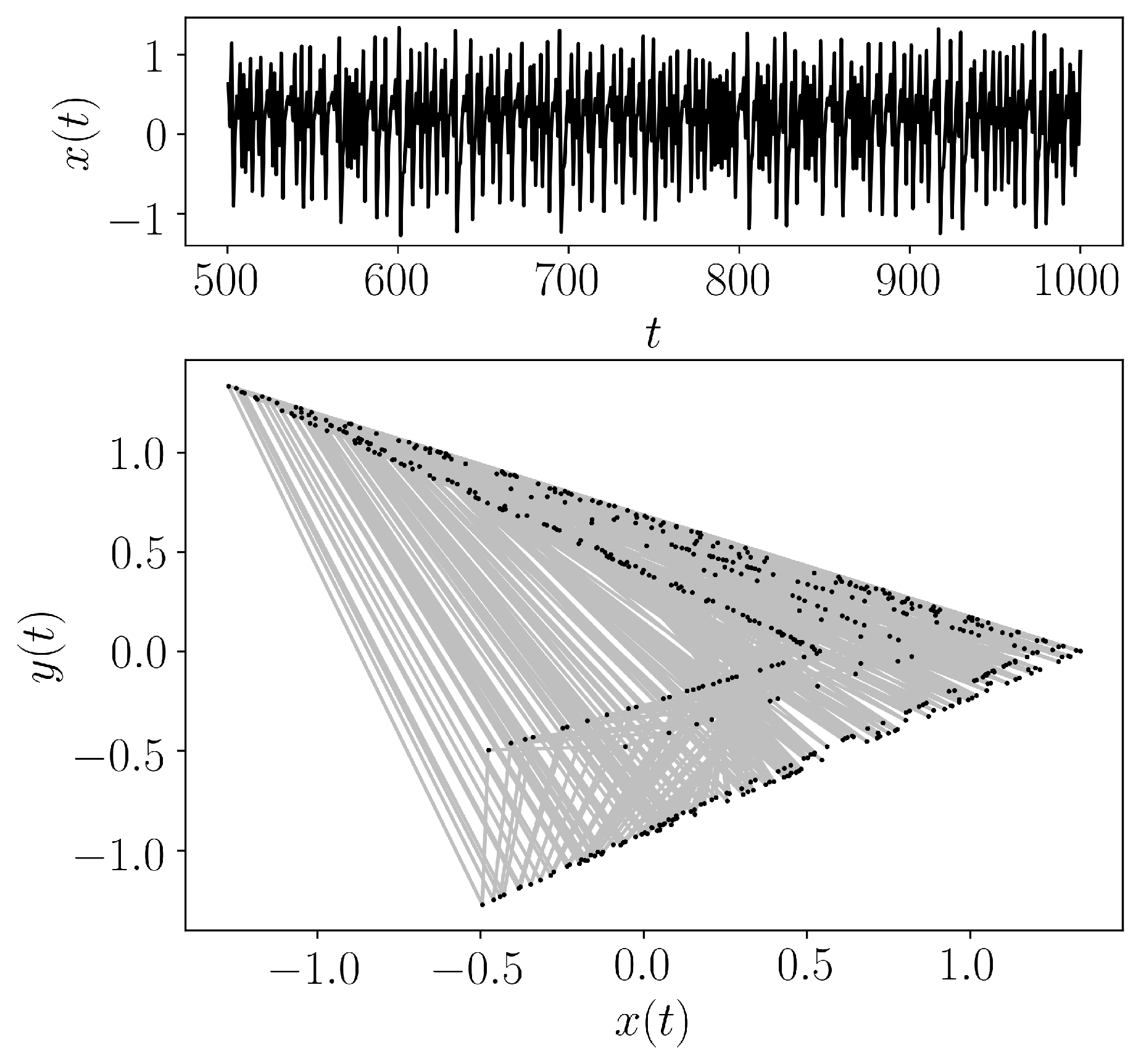
- teaspoon.MakeData.DynSysLib.maps.tinkerbell_map(parameters=[0.7, -0.6, 2, 0.5], dynamic_state=None, InitialConditions=None, L=1000.0, fs=1, SampleSize=500)[source]
The Tinkerbell map is defined [11] as
\[ \begin{align}\begin{aligned}x_{n+1} &= x_n^2 - y_n^2 + ax_n + by_n,\\y_{n+1} &= 2x_ny_n + cx_n + dy_n\end{aligned}\end{align} \]where we chose the parameters \(a = 0.9\), \(b = -0.6\), \(c = 2.0\), and \(d = 0.5\) for a chaotic state with initial conditions \(x_0 = 0.0\) and \(y_0 = 0.5\). You can set \(a = 0.7\) for a periodic response. We solve this system for 1000 data points and keep the second 500 to avoid transients.
- Parameters:
parameters (Optional[float]) – Array of system parameters [a,b,c,d].
dynamic_state (Optional[string]) – Dynamic state (‘periodic’ or ‘chaotic’)
L (Optional[int]) – Number of map iterations.
fs (Optional[int]) – sampling rate for simulation.
SampleSize (Optional[int]) – length of sample at end of entire time series
- Returns:
Array of the time indices as t and the simulation time series ts
- Return type:
array
References
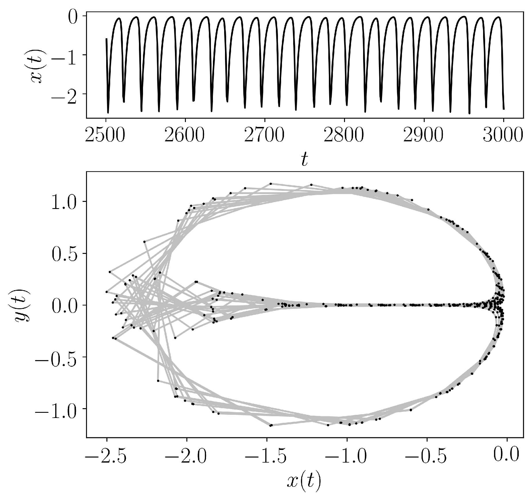
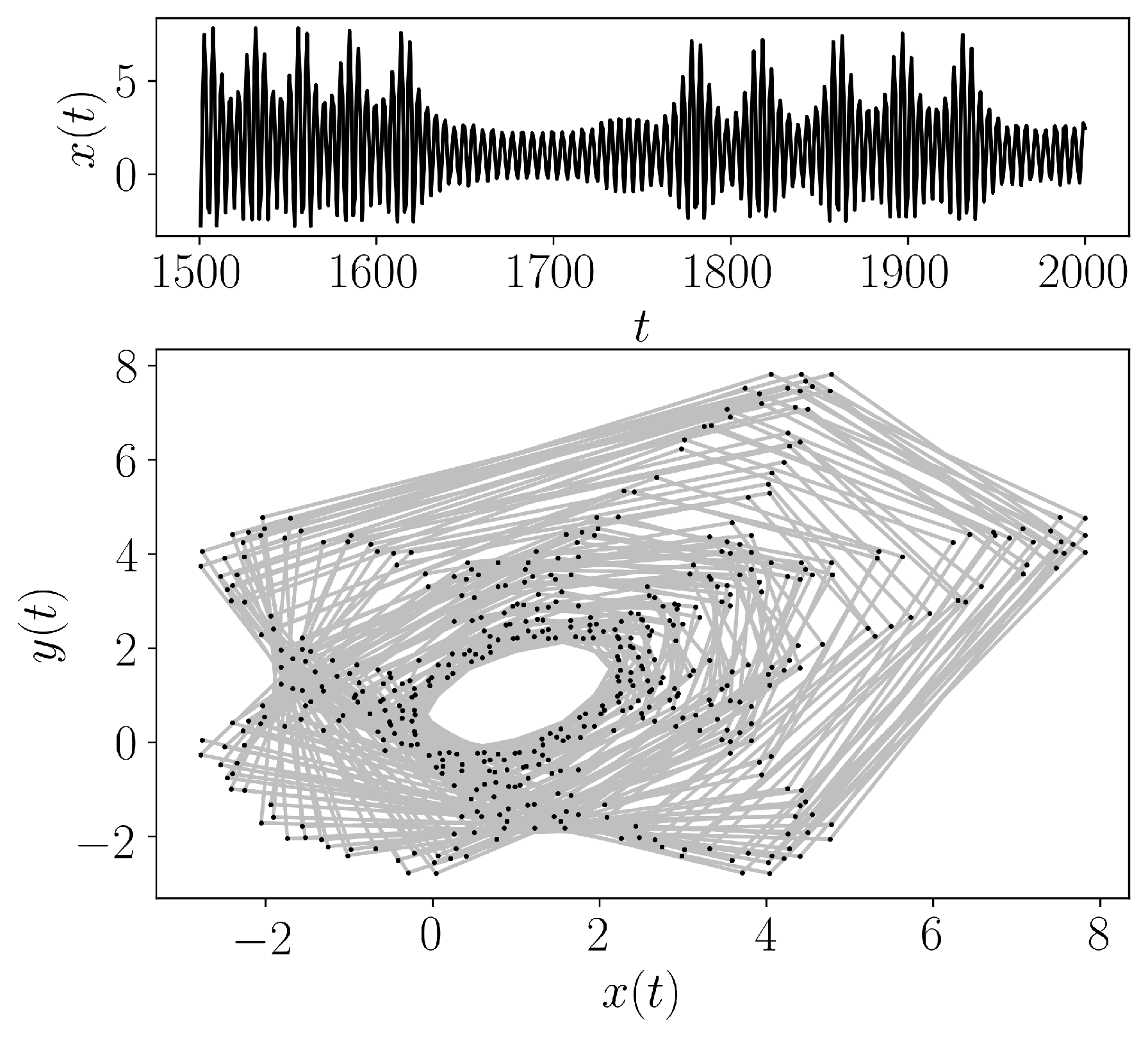
- teaspoon.MakeData.DynSysLib.maps.burgers_map(parameters=[0.75, 1.6], dynamic_state=None, InitialConditions=None, L=3000.0, fs=1, SampleSize=500)[source]
The Burger’s map is defined [12] as
\[ \begin{align}\begin{aligned}x_{n+1} &= ax_n - y_n^2,\\y_{n+1} &= by_n + x_ny_n\end{aligned}\end{align} \]where we chose the parameters \(a = 0.75\) and \(b = 1.75\) for a chaotic state with initial conditions \(x_0 = -0.1\) and \(y_0 = 0.5\). You can set \(b = 1.60\) for a periodic response. We solve this system for 3000 data points and keep the second 500 to avoid transients.
- Parameters:
parameters (Optional[float]) – Array of system parameters [a,b].
dynamic_state (Optional[string]) – Dynamic state (‘periodic’ or ‘chaotic’)
L (Optional[int]) – Number of map iterations.
fs (Optional[int]) – sampling rate for simulation.
SampleSize (Optional[int]) – length of sample at end of entire time series
- Returns:
Array of the time indices as t and the simulation time series ts
- Return type:
array
References
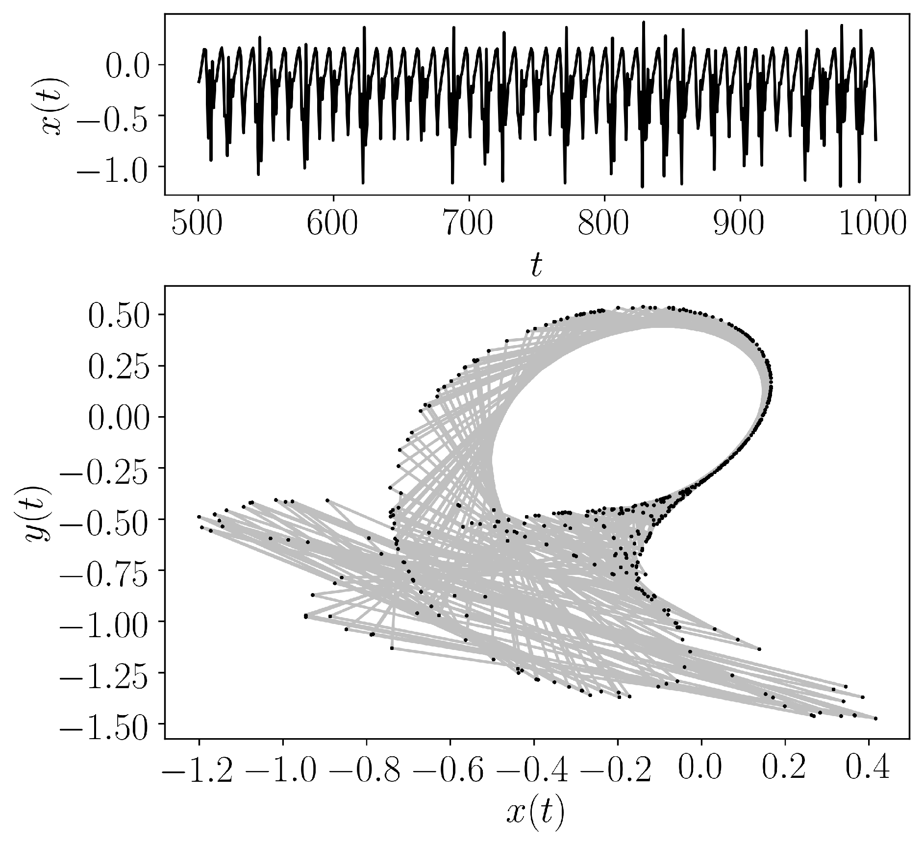
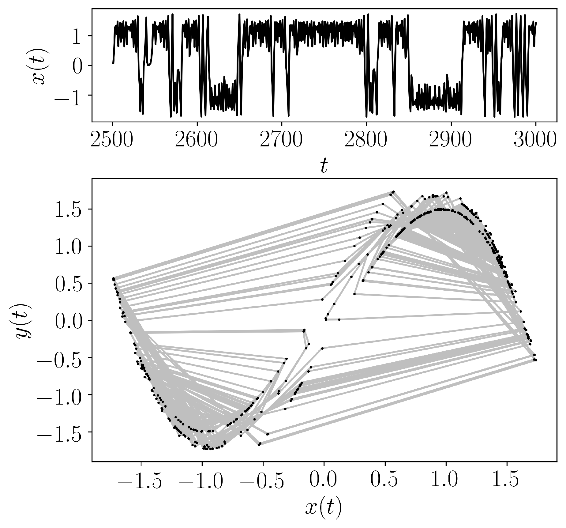
- teaspoon.MakeData.DynSysLib.maps.holmes_cubic_map(parameters=[0.27, 2.77], dynamic_state=None, InitialConditions=None, L=3000.0, fs=1, SampleSize=500)[source]
The Holme’s Cubic map is defined [13] as
\[ \begin{align}\begin{aligned}x_{n+1} &= y_n,\\y_{n+1} &= -bx_n + dy_n - y_n^3\end{aligned}\end{align} \]where we chose the parameters \(b = 0.20\) and \(d = 2.77\) for a chaotic state with initial conditions \(x_0 = -0.1\) and \(y_0 = 0.5\). You can set \(b = 0.27\) for a periodic response. We solve this system for 3000 data points and keep the second 500 to avoid transients.
- Parameters:
parameters (Optional[float]) – Array of system parameters [b,d].
dynamic_state (Optional[string]) – Dynamic state (‘periodic’ or ‘chaotic’)
L (Optional[int]) – Number of map iterations.
fs (Optional[int]) – sampling rate for simulation.
SampleSize (Optional[int]) – length of sample at end of entire time series
- Returns:
Array of the time indices as t and the simulation time series ts
- Return type:
array
References
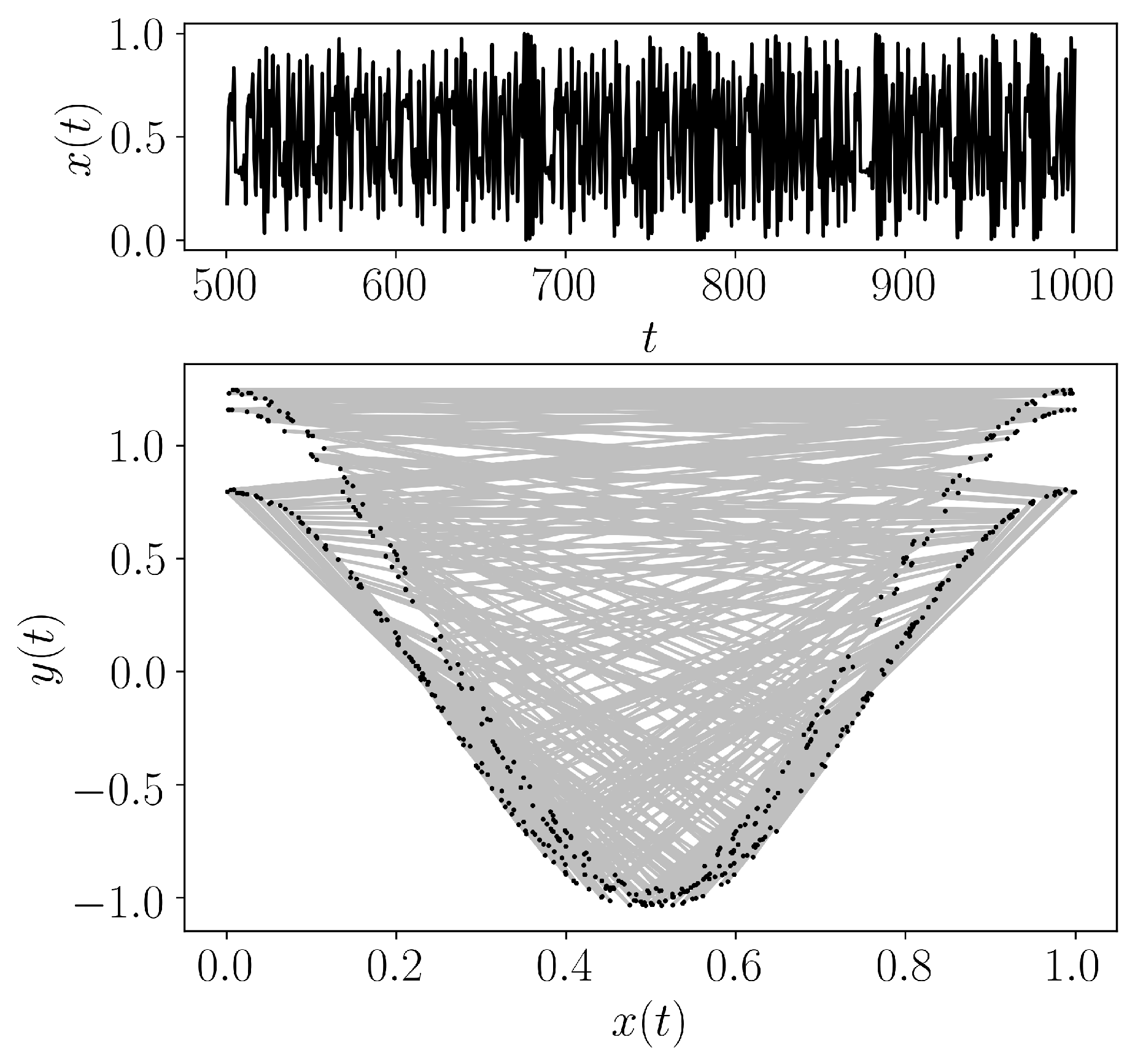
- teaspoon.MakeData.DynSysLib.maps.kaplan_yorke_map(parameters=[-1.0, 0.2], dynamic_state=None, InitialConditions=None, L=1000.0, fs=1, SampleSize=500)[source]
The Kaplan Yorke map is defined [14] as
\[ \begin{align}\begin{aligned}x_{n+1} &= [ax_n](\mod 1),\\y_{n+1} &= by_n + \cos{(4\pi x_n)}\end{aligned}\end{align} \]where we chose the parameters \(a = -2.0\) and \(b = 0.2\) for a chaotic state with initial conditions \(x_0 = -0.1\) and \(y_0 = 0.5\). You can set \(a = -1.0\) for a periodic response. We solve this system for 1000 data points and keep the second 500 to avoid transients.
- Parameters:
parameters (Optional[float]) – Array of system parameters [a,b].
dynamic_state (Optional[string]) – Dynamic state (‘periodic’ or ‘chaotic’)
L (Optional[int]) – Number of map iterations.
fs (Optional[int]) – sampling rate for simulation.
SampleSize (Optional[int]) – length of sample at end of entire time series
- Returns:
Array of the time indices as t and the simulation time series ts
- Return type:
array
References
- teaspoon.MakeData.DynSysLib.maps.gingerbread_man_map(parameters=[1.0, 1.0], dynamic_state=None, InitialConditions=None, L=2000, fs=1, SampleSize=500)[source]
The Gingerbread Man Map is defined [15] [16] as
\[ \begin{align}\begin{aligned}x_{n+1} &= 1 - ay_n + n|x_n|,\\y_{n+1} &= x_n\end{aligned}\end{align} \]where we chose the parameters \(a = 1.0\) and \(b = 1.0\). For a chaotic state, initial conditions \(x_0 = 0.5\) and \(y_0 = 1.8\), and for a periodic response \(x_0 = 0.5\) and \(y_0 = 1.5\). We solve this system for 2000 data points and keep the last 500 to avoid transients.
- Parameters:
a (Optional[float]) – System parameter.
b (Optional[float]) – System parameter.
dynamic_state (Optional[string]) – Dynamic state (‘periodic’ or ‘chaotic’)
L (Optional[int]) – Number of map iterations.
fs (Optional[int]) – sampling rate for simulation.
SampleSize (Optional[int]) – length of sample at end of entire time series
- Returns:
Array of the time indices as t and the simulation time series ts
- Return type:
array
References