2.1.2.2. Autonomous Dissipative Flows

2.1.2.2.1. Main Functions

teaspoon.MakeData.DynSysLib.autonomous_dissipative_flows.lorenz(parameters=[100, 10, 2.6666666666666665], dynamic_state=None, InitialConditions=[1e-10, 0.0, 1.0], L=100.0, fs=100, SampleSize=2000)

The Lorenz system used is defined as

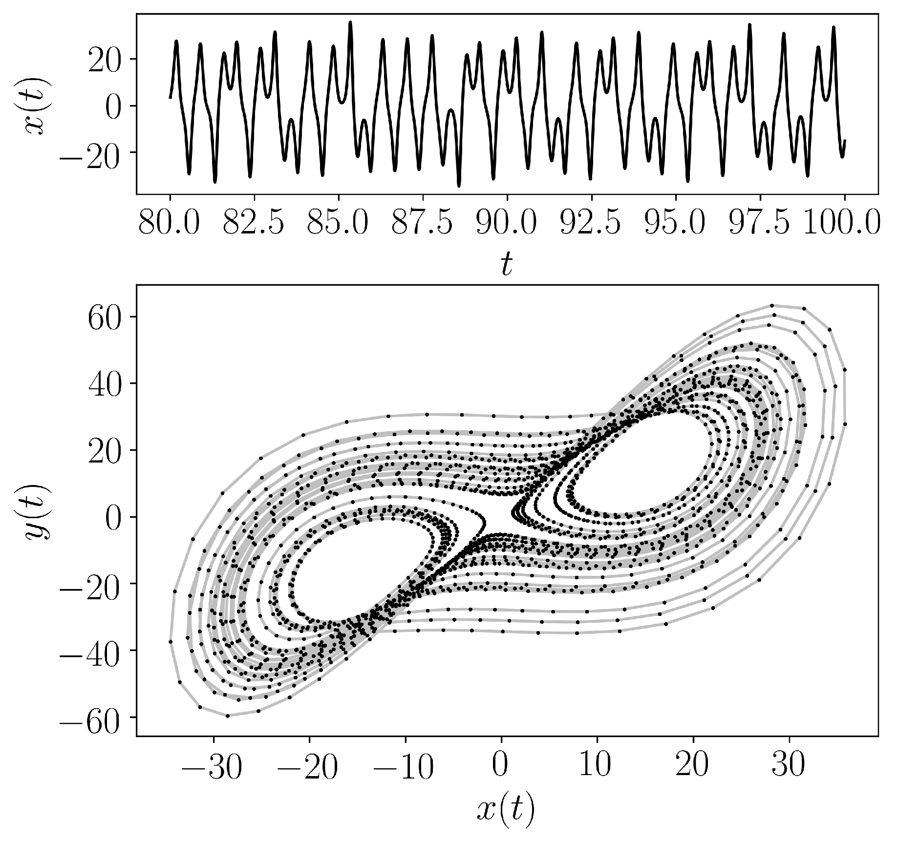
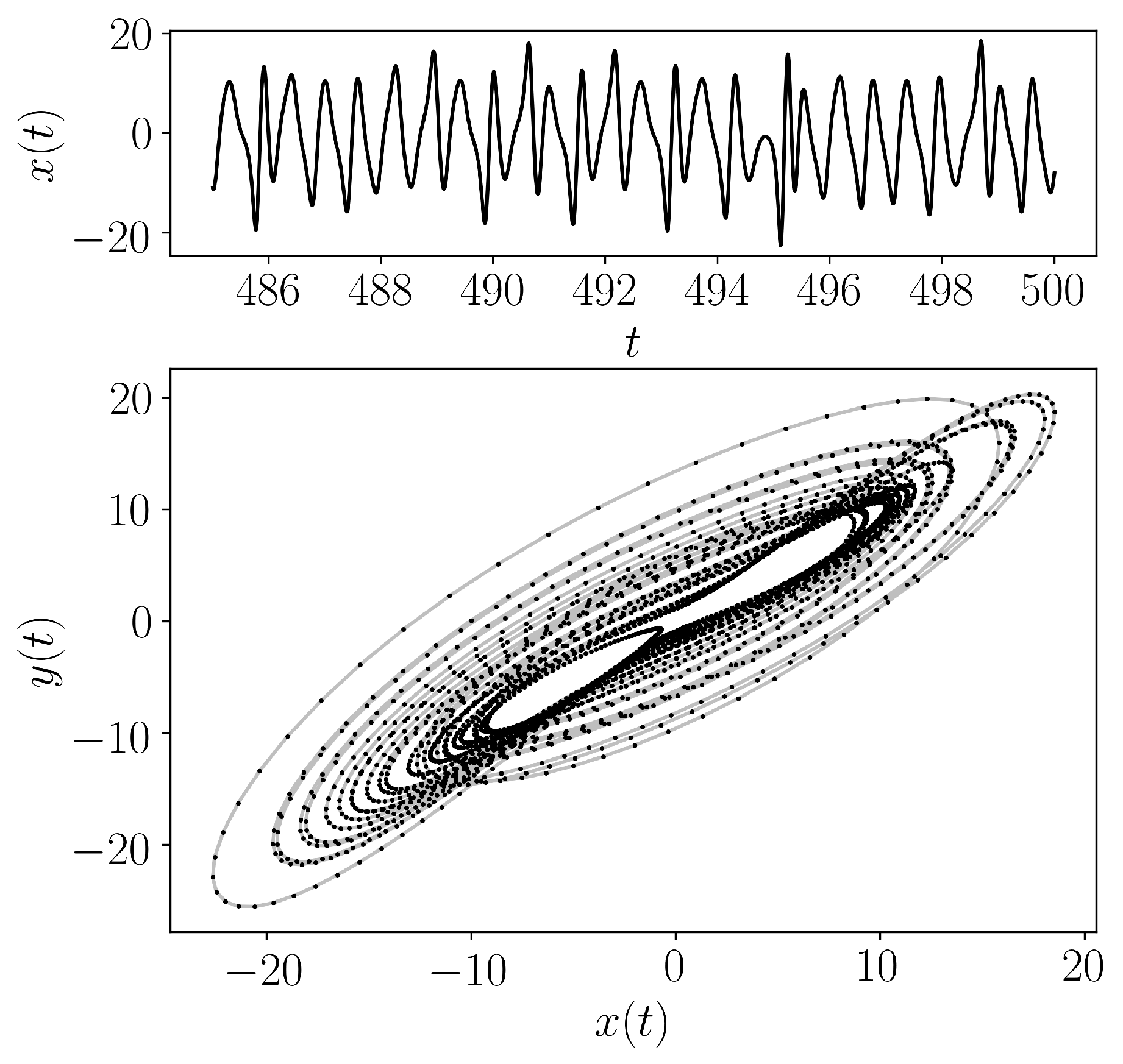
\[ \begin{align}\begin{aligned}\dot{x} &= \sigma (y - x),\\\dot{y} &= x (\rho - z) - y,\\\dot{z} &= x y - \beta z\end{aligned}\end{align} \]

The Lorenz system was solved with a sampling rate of 100 Hz for 100 seconds with only the last 20 seconds used to avoid transients. For a chaotic response, parameters of \(\sigma = 10.0\), \(\beta = 8.0/3.0\), and \(\rho = 105\) and initial conditions \([x_0,y_0,z_0] = [10^{-10},0,1]\) are used. For a periodic response set \(\rho = 100\).

Parameters:

• parameters (Optional[floats]) – Array of three floats [\(\rho\), \(\sigma\), \(\beta\)] or None if using the dynamic_state variable

• fs (Optional[float]) – Sampling rate for simulation

• SampleSize (Optional[int]) – length of sample at end of entire time series

• L (Optional[int]) – Number of iterations

• InitialConditions (Optional[floats]) – list of values for [\(x_{0}\), \(y_{0}\), \(z_{0}\)]

• dynamic_state (Optional[str]) – Set dynamic state as either ‘periodic’ or ‘chaotic’ if not supplying parameters.

Returns:

Array of the time indices as t and the simulation time series ts

Return type:

array

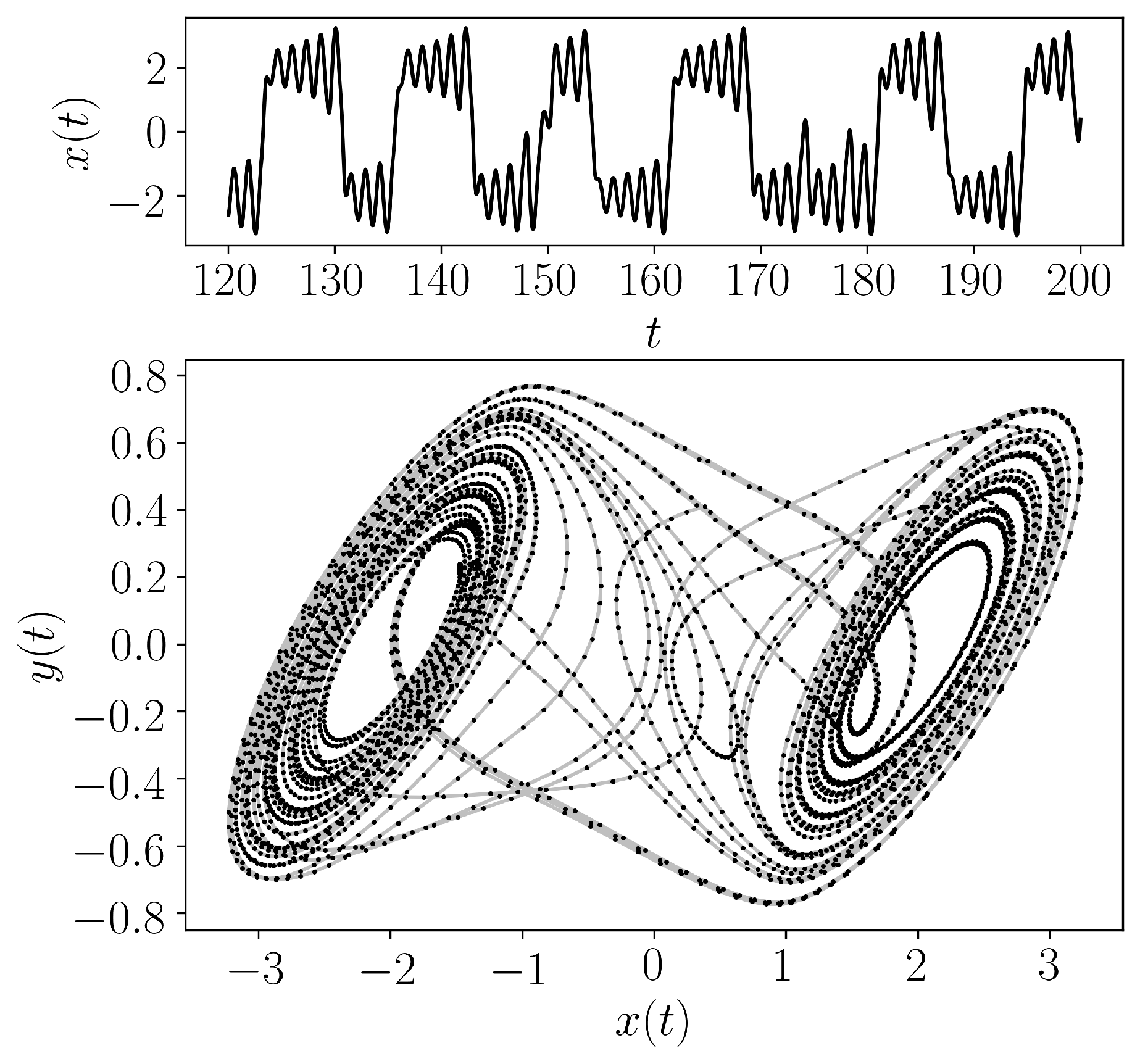
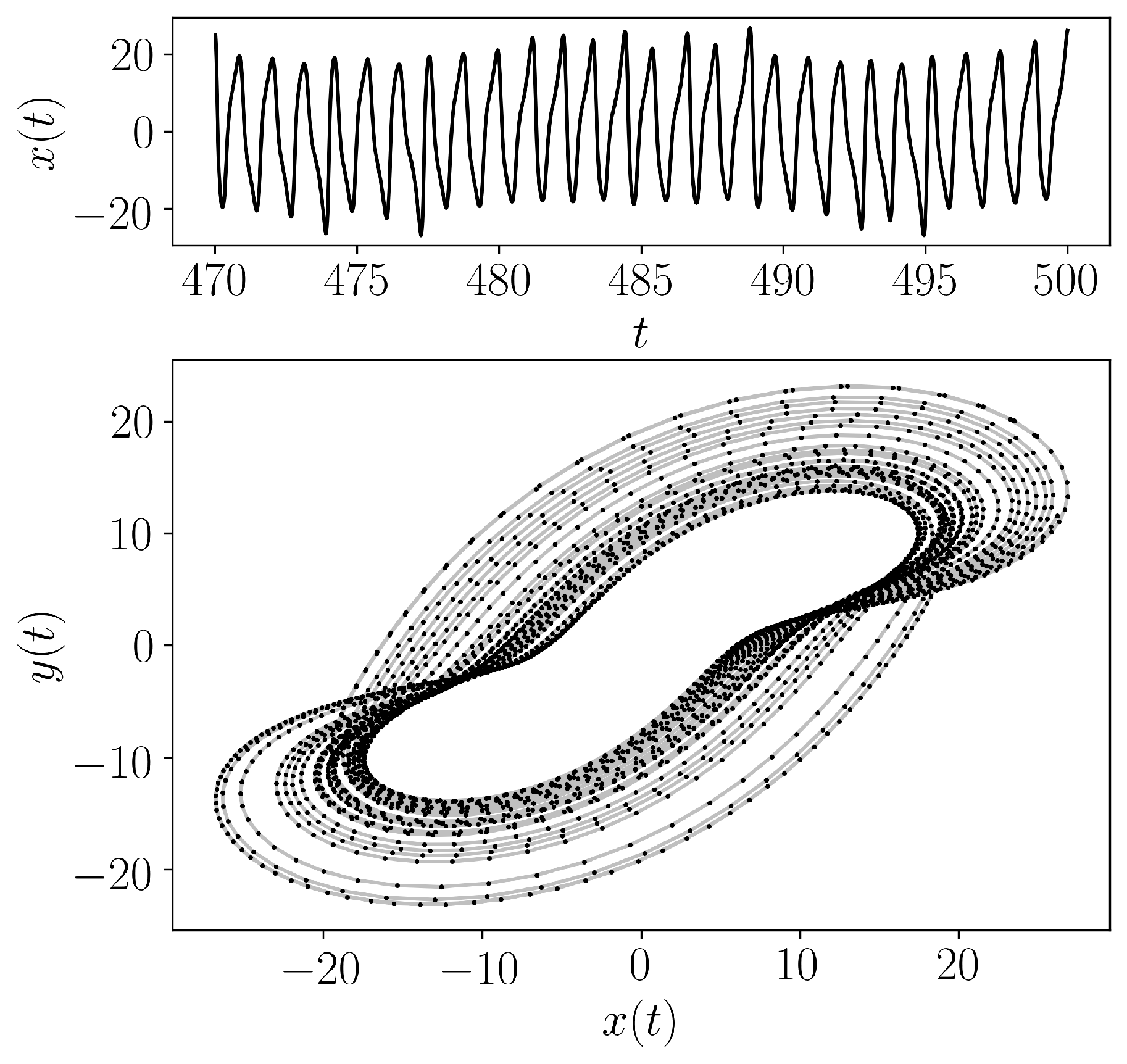
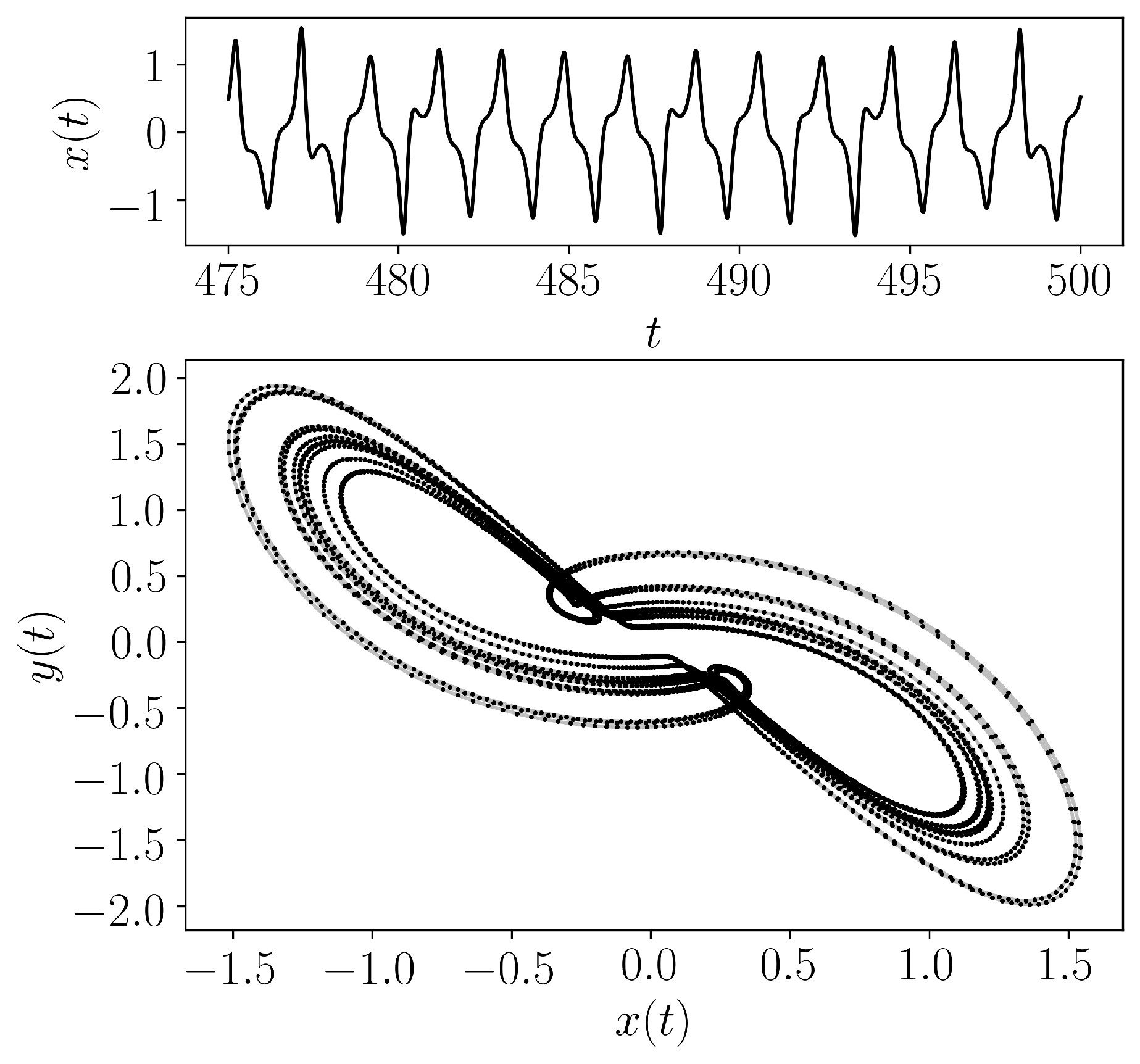
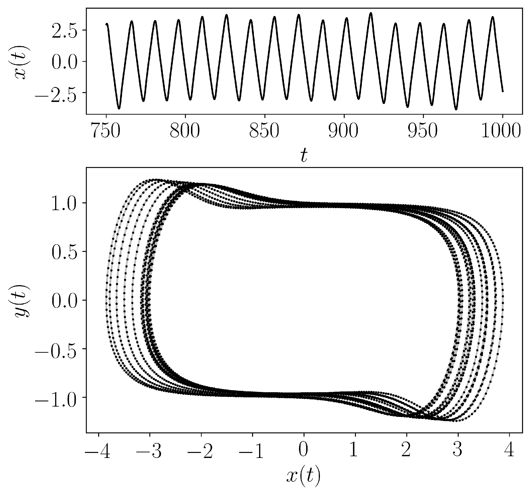
teaspoon.MakeData.DynSysLib.autonomous_dissipative_flows.rossler(parameters=[0.1, 0.2, 14], dynamic_state=None, InitialConditions=[-0.4, 0.6, 1], L=1000.0, fs=15, SampleSize=2500)

The Rössler system used was defined as

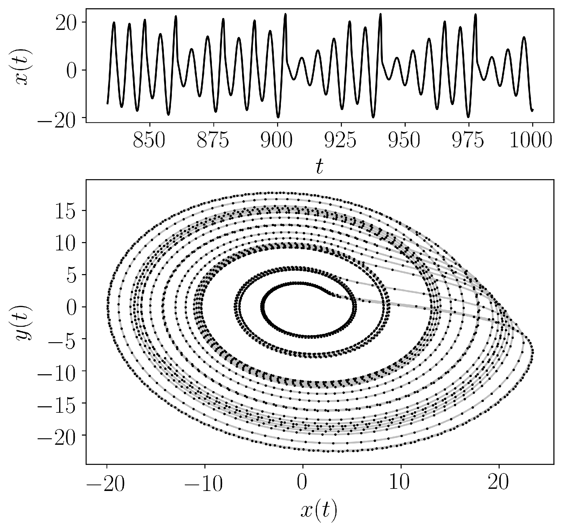
\[ \begin{align}\begin{aligned}\dot{x} &= -y-z,\\\dot{y} &= x + ay,\\\dot{z} &= b + z(x-c)\end{aligned}\end{align} \]

The Rössler system was solved with a sampling rate of 15 Hz for 1000 seconds with only the last 166 seconds used to avoid transients. For a chaotic response, parameters of \(a = 0.15\), \(b = 0.2\), and \(c = 14\) and initial conditions \([x_0,y_0,z_0] = [-0.4,0.6,1.0]\) are used. For a periodic response set \(a = 0.10\).

Parameters:

• parameters (Optional[floats]) – Array of three floats [a, b, c] or None if using the dynamic_state variable

• fs (Optional[float]) – Sampling rate for simulation

• SampleSize (Optional[int]) – length of sample at end of entire time series

• L (Optional[int]) – Number of iterations

• InitialConditions (Optional[floats]) – list of values for [\(x_{0}\), \(y_{0}\), \(z_{0}\)]

• dynamic_state (Optional[str]) – Set dynamic state as either ‘periodic’ or ‘chaotic’ if not supplying parameters.

Returns:

Array of the time indices as t and the simulation time series ts

Return type:

array

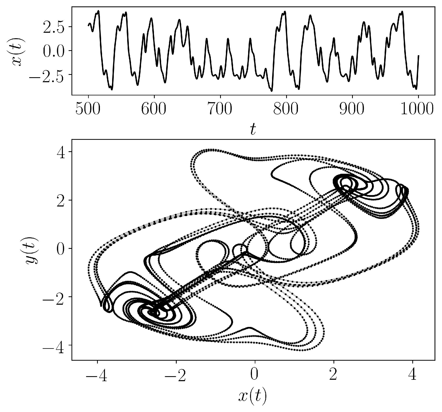
teaspoon.MakeData.DynSysLib.autonomous_dissipative_flows.coupled_lorenz_rossler(parameters=[0.25, 2.6666666666666665, 0.2, 5.7, 0.1, 0.1, 0.1, 28, 10], dynamic_state=None, InitialConditions=[0.1, 0.1, 0.1, 0, 0, 0], L=500.0, fs=50, SampleSize=15000)

The coupled Lorenz-Rössler system is defined as

\[ \begin{align}\begin{aligned}\dot{x}_1 &= -y_1-z_1+k_1(x_2-x_1),\\\dot{y}_1 &= x_1 + ay_1+k_2(y_2-y_1),\\\dot{z}_1 &= b_2 + z_1(x_1-c_2) + k_3(z_2-z_1),\\\dot{x}_2 &= \sigma (y_2-x_2),\\\dot{y}_2 &= \lambda x_2 - y_2 - x_2z_2,\\\dot{z}_2 &= x_2y_2 - b_1z_2\end{aligned}\end{align} \]

where \(b_1 =8/3\), \(b_2 =0.2\), \(c_2 =5.7\), \(k_1 =0.1\), \(k_2 =0.1\), \(k_3 =0.1\), \(\lambda =28\), \(\sigma =10\),and \(a=0.25\) for a periodic response and \(a = 0.51\) for a chaotic response. This system was simulated at a frequency of 50 Hz for 500 seconds with the last 300 seconds used. The default initial condition is \([x_1, y_1, z_1, x_2, y_2, z_2]=[0.1,0.1,0.1,0,0,0]\).

Parameters:

• parameters (Optional[floats]) – Array of nine floats [\(a\), \(b_1\), \(b_2\), \(c_2\), \(k_1\), \(k_2\), \(k_3\), \(\lambda\), \(\sigma\)] or None if using the dynamic_state variable

• fs (Optional[float]) – Sampling rate for simulation

• SampleSize (Optional[int]) – length of sample at end of entire time series

• L (Optional[int]) – Number of iterations

• InitialConditions (Optional[floats]) – list of values for [\(x_{1, 0}\), \(y_{1, 0}\), \(z_{1, 0}\), \(x_{2, 0}\), \(y_{2, 0}\), \(z_{2, 0}\)]

• dynamic_state (Optional[str]) – Set dynamic state as either ‘periodic’ or ‘chaotic’ if not supplying parameters.

Returns:

Array of the time indices as t and the simulation time series ts

Return type:

array

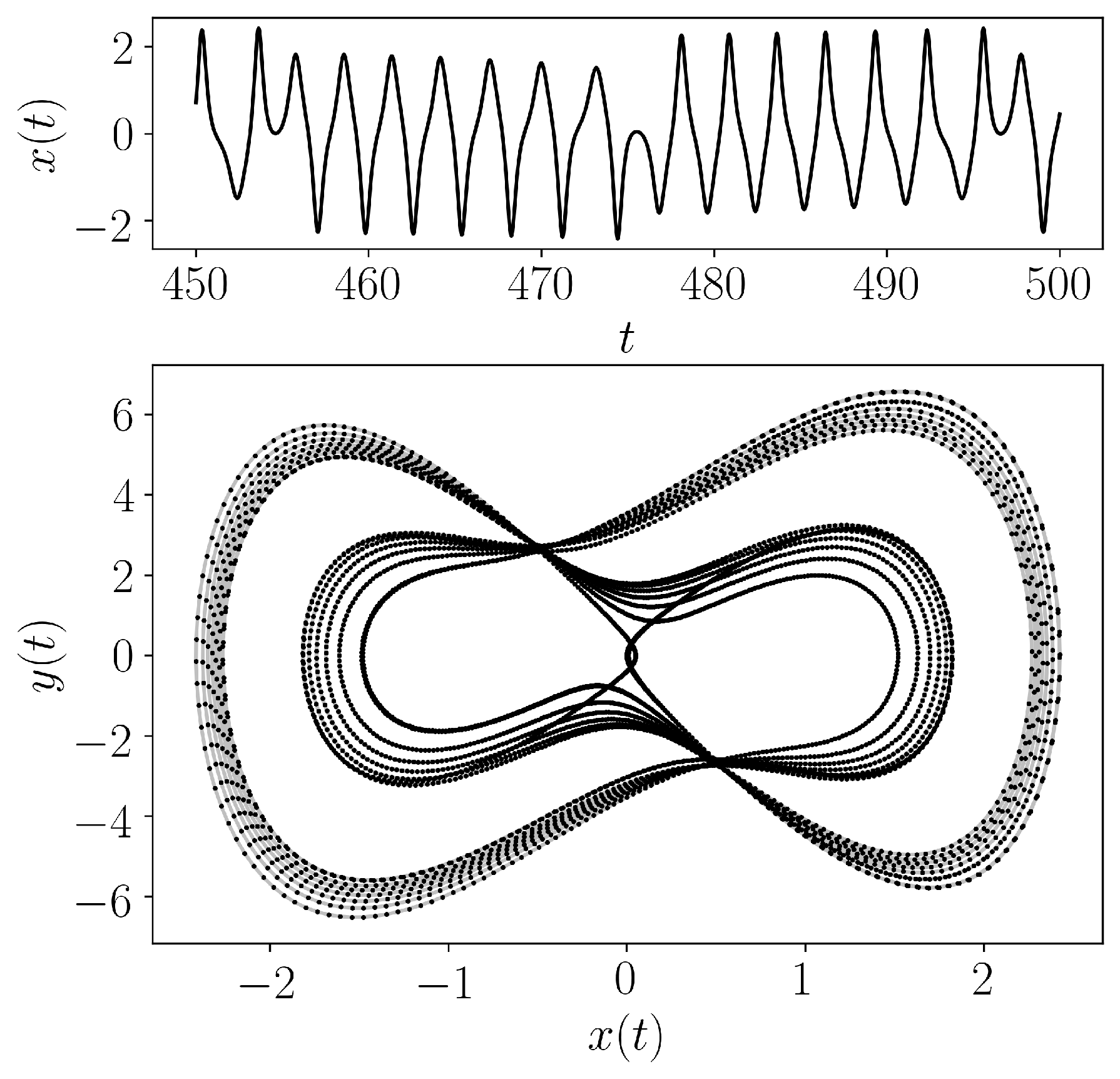
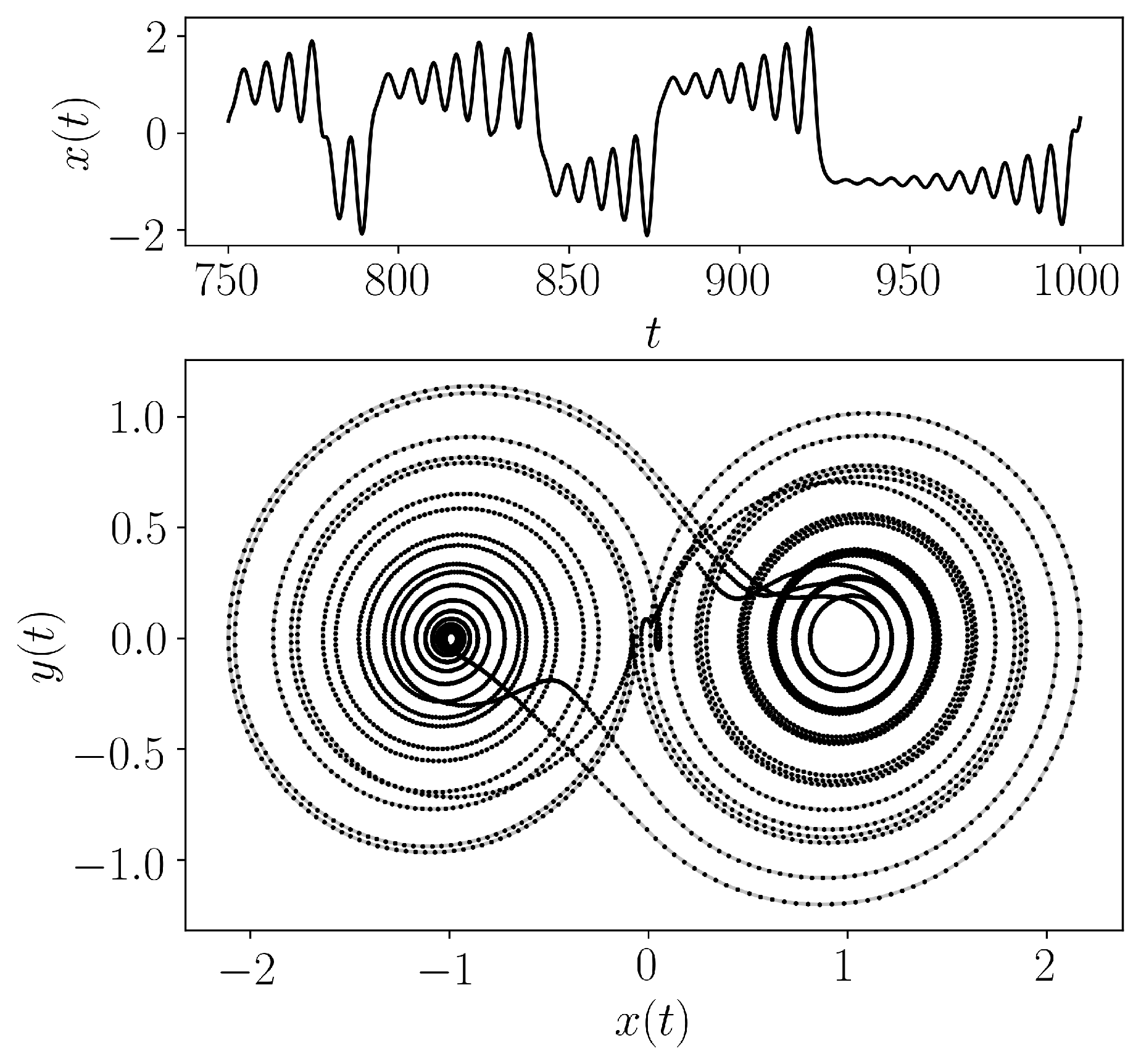
teaspoon.MakeData.DynSysLib.autonomous_dissipative_flows.coupled_rossler_rossler(parameters=[0.25, 0.99, 0.95], dynamic_state=None, InitialConditions=[-0.4, 0.6, 5.8, 0.8, -2, -4], L=1000.0, fs=10, SampleSize=1500)

The coupled Lorenz-Rössler system is defined as

\[ \begin{align}\begin{aligned}\dot{x}_1 &= -w_1y_1 - z_1 +k(x_2-x_1),\\\dot{y}_1 &= w_1x_1 + 0.165y_1,\\\dot{z}_1 &= 0.2 + z_1(x_1-10),\\\dot{x}_2 &= -w_2y_2-z_2 + k(x_1-x_2),\\\dot{y}_2 &= w_2x_2 + 0.165y_2,\\\dot{z}_2 &= 0.2 + z_2(x_2-10)\end{aligned}\end{align} \]

with \(w_1 = 0.99\), \(w_2 = 0.95\), and \(k = 0.05\). This was solved for 1000 seconds with a sampling rate of 10 Hz. Only the last 150 seconds of the solution are used and the default initial condition is \([x_1, y_1, z_1, x_2, y_2, z_2]=[-0.4,0.6,5.8,0.8,-2,-4]\).

Parameters:

• parameters (Optional[floats]) – Array of three floats [\(k\), \(w_1\), \(w_2\)] or None if using the dynamic_state variable

• fs (Optional[float]) – Sampling rate for simulation

• SampleSize (Optional[int]) – length of sample at end of entire time series

• L (Optional[int]) – Number of iterations

• InitialConditions (Optional[floats]) – list of values for [\(x_{1, 0}\), \(y_{1, 0}\), \(z_{1, 0}\), \(x_{2, 0}\), \(y_{2, 0}\), \(z_{2, 0}\)]

• dynamic_state (Optional[str]) – Set dynamic state as either ‘periodic’ or ‘chaotic’ if not supplying parameters.

Returns:

Array of the time indices as t and the simulation time series ts

Return type:

array

teaspoon.MakeData.DynSysLib.autonomous_dissipative_flows.chua(parameters=[10.8, 27, 1.0, -0.42857142857142855, 0.42857142857142855], dynamic_state=None, InitialConditions=[1.0, 0.0, 0.0], L=200.0, fs=50, SampleSize=4000)

Chua’s circuit is based on a non-linear circuit and is described as

\[ \begin{align}\begin{aligned}\dot{x} &= \alpha (y-f(x)),\\\dot{y} &= \gamma (x-y+z),\\\dot{z} &= -\beta y,\end{aligned}\end{align} \]

where \(f(x)\) is based on a non-linear resistor model defined as

\[f(x) = m_1x + \frac{1}{2}(m_0+m_1)[|x+1| - |x-1|]\]

The system parameters are set to \(\beta=27\), \(\gamma=1\), \(m_0 =-3/7\), \(m_1 =3/7\), and \(\alpha=10.8\) for a periodic response and \(\alpha = 12.8\) for a chaotic response. The system was simulated for 200 seconds at a rate of 50 Hz and the last 80 seconds are used.

Parameters:

• parameters (Optional[floats]) – Array of five floats [\(a\), \(B\), \(g\), \(m_0\), \(m_1\)] or None if using the dynamic_state variable

• fs (Optional[float]) – Sampling rate for simulation

• SampleSize (Optional[int]) – length of sample at end of entire time series

• L (Optional[int]) – Number of iterations

• InitialConditions (Optional[floats]) – list of values for [\(x_0\), \(y_0\), \(z_0\)]

• dynamic_state (Optional[str]) – Set dynamic state as either ‘periodic’ or ‘chaotic’ if not supplying parameters.

Returns:

Array of the time indices as t and the simulation time series ts

Return type:

array

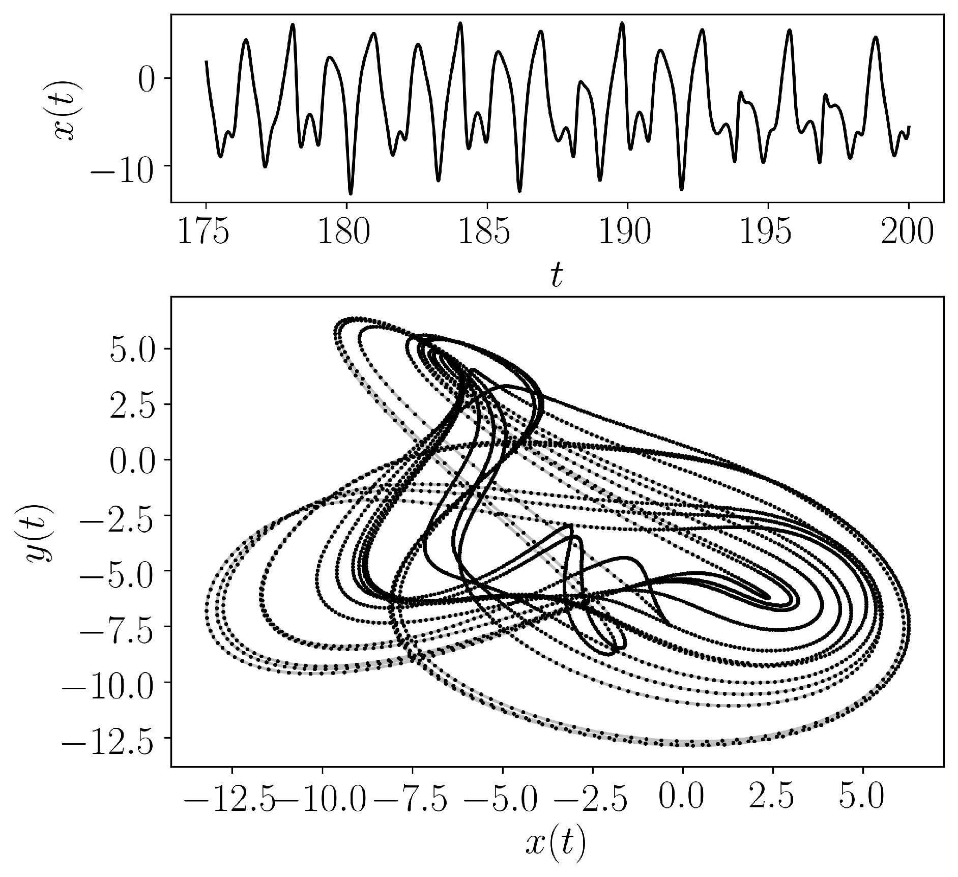
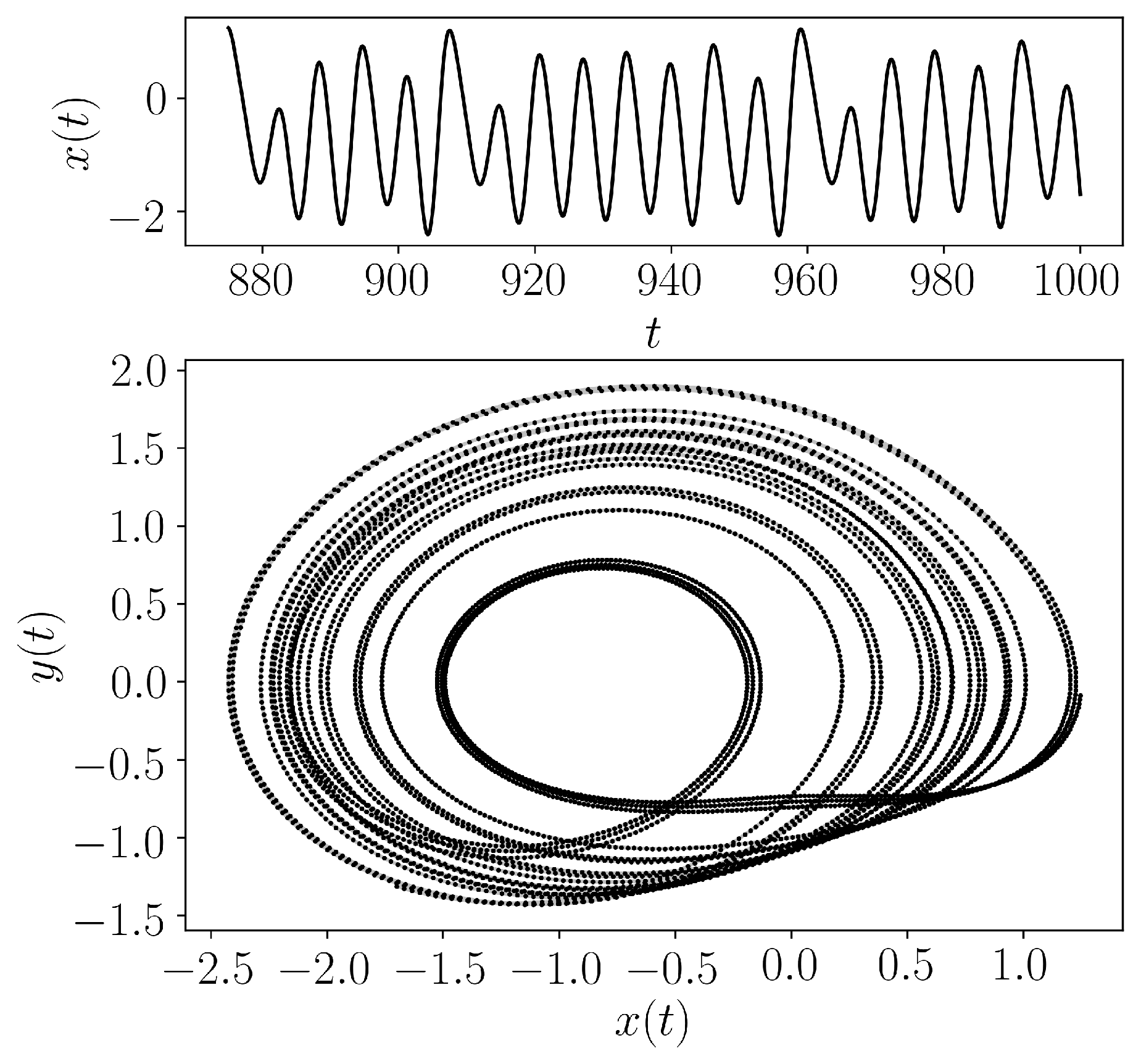
teaspoon.MakeData.DynSysLib.autonomous_dissipative_flows.double_pendulum(parameters=[1, 1, 1, 1, 9.81], dynamic_state=None, InitialConditions=[0.4, 0.6, 1, 1], L=100.0, fs=100, SampleSize=5000)

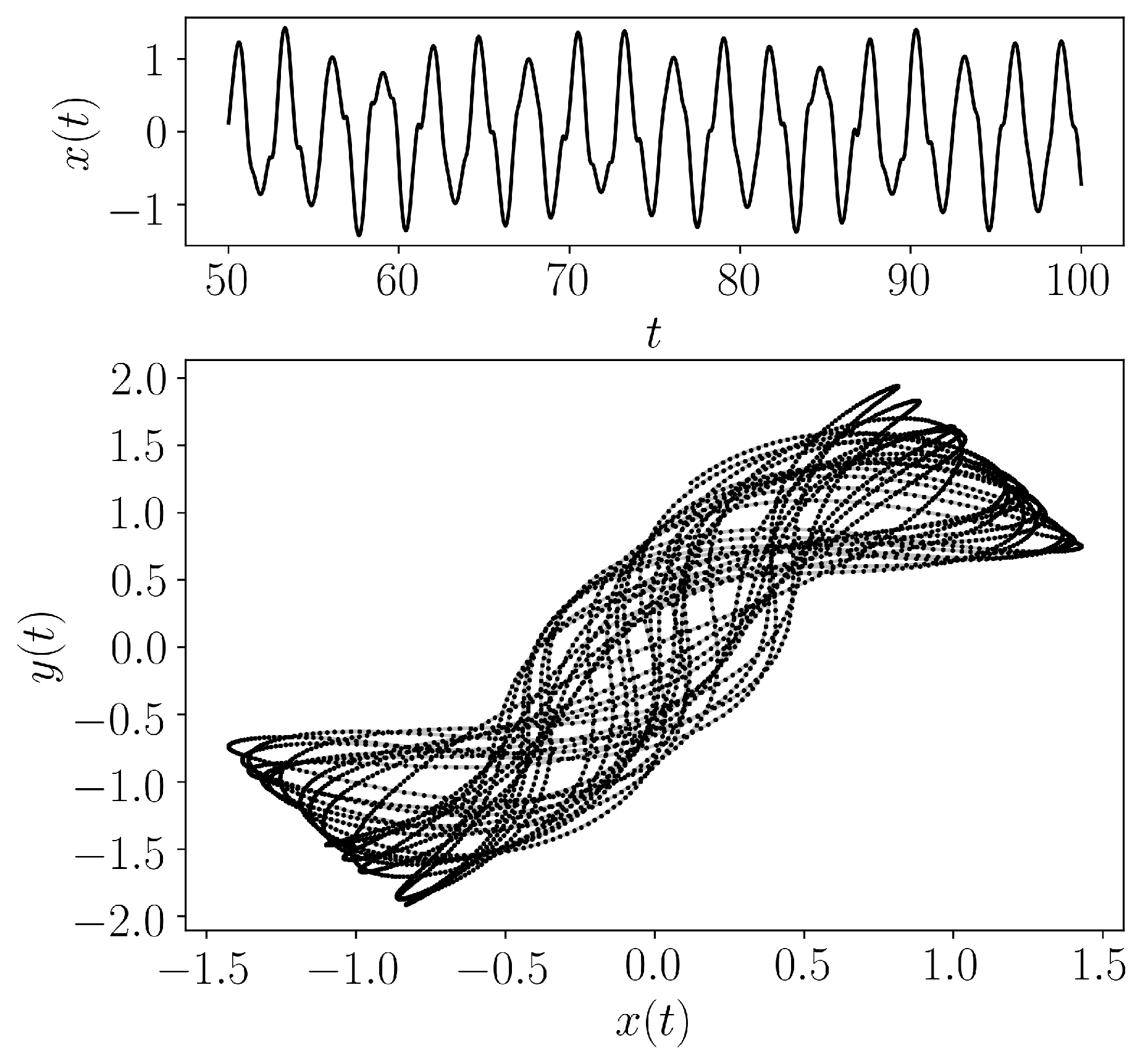
The double pendulum is a staple bench top experiment for investigated chaos in a mechanical system. A point-mass double pendulum’s equations of motion are defined as

\[ \begin{align}\begin{aligned}\dot{\theta}_1 &= \omega_1,\\\dot{\theta}_2 &= \omega_2,\\\dot{\omega}_1 &= \frac{-g(2m_1+m_2)\sin(\theta_1) - m_2g\sin(\theta_1-2\theta_2) - 2\sin(\theta_1-\theta2)m_2(\omega_2^2 l_2 + \omega_1^2 l_1\cos(\theta_1-\theta_2))}{l_1(2m_1+m_2-m_2\cos(2\theta_1-2\theta_2))},\\\dot{\omega}_2 &= \frac{2\sin(\theta_1-\theta_2)(\omega_1^2 l_1(m_1+m_2)+g(m_1+m_2)\cos(\theta_1)+\omega_2^2 l_2m_2\cos(\theta_1-\theta_2))}{l_2(2m_1+m_2-m_2\cos(2\theta_1-2\theta_2))}\end{aligned}\end{align} \]

where the system parameters are \(g=9.81 m/s^2\), \(m_1 =1 kg\), \(m_2 =1 kg\), \(l_1 = 1 m\), and \(l_2 =1 m\). The system was solved for 200 seconds at a rate of 100 Hz and only the last 30 seconds were used as shown in the figure below for the chaotic response with initial conditions \([\theta_1, \theta_2, \omega_1, \omega_2] = [0, 3 rad, 0, 0]\). This system will have different dynamic states based on the initial conditions, which can vary from periodic, quasiperiodic, and chaotic.

Parameters:

• parameters (Optional[floats]) – Array of five floats [\(m_1\), \(m_2\), \(l_1\), \(l_2\), \(g\)] or None if using the dynamic_state variable

• fs (Optional[float]) – Sampling rate for simulation

• SampleSize (Optional[int]) – length of sample at end of entire time series

• L (Optional[int]) – Number of iterations

• InitialConditions (Optional[floats]) – list of values for [\(\theta_{1, 0}\), \(\theta_{2, 0}\), \(\omega_{1, 0}\), \(\omega_{2, 0}\)]

• dynamic_state (Optional[str]) – Set dynamic state as either ‘periodic’ or ‘chaotic’ if not supplying parameters.

Returns:

Array of the time indices as t and the simulation time series ts

Return type:

array

teaspoon.MakeData.DynSysLib.autonomous_dissipative_flows.diffusionless_lorenz_attractor(parameters=[0.25], dynamic_state=None, InitialConditions=[1, -1, 0.01], L=1000.0, fs=40, SampleSize=10000)

The Diffusionless Lorenz attractor is defined as

\[ \begin{align}\begin{aligned}\dot{x} &= -y-x,\\\dot{y} &= -xz,\\\dot{z} &= xy + R\end{aligned}\end{align} \]

The system parameter is set to \(R = 0.40\) for a chaotic response and \(R = 0.25\) for a periodic response. The initial conditions were set to \([x, y, z] = [1.0, -1.0, 0.01]\). The system was simulated for 1000 seconds at a rate of 40 Hz and the last 250 seconds were used for the chaotic response.

Parameters:

• parameters (Optional[floats]) – Array of one float [\(R\)] or None if using the dynamic_state variable

• fs (Optional[float]) – Sampling rate for simulation

• SampleSize (Optional[int]) – length of sample at end of entire time series

• L (Optional[int]) – Number of iterations

• InitialConditions (Optional[floats]) – list of values for [\(x_0\), \(y_0\), \(z_0\)]

• dynamic_state (Optional[str]) – Set dynamic state as either ‘periodic’ or ‘chaotic’ if not supplying parameters.

Returns:

Array of the time indices as t and the simulation time series ts

Return type:

array

teaspoon.MakeData.DynSysLib.autonomous_dissipative_flows.complex_butterfly(parameters=[0.15], dynamic_state=None, InitialConditions=[0.2, 0.0, 0.0], L=1000.0, fs=10, SampleSize=5000)

The Complex Butterfly attractor [1] is defined as

\[ \begin{align}\begin{aligned}\dot{x} &= a(y-x),\\\dot{y} &= z~\text{sgn}(x),\\\dot{z} &= |x|-1\end{aligned}\end{align} \]

The system parameter is set to \(a = 0.55\) for a chaotic response and \(a = 0.15\) for a periodic response. The initial conditions were set to \([x, y, z] = [0.2, 0.0, 0.0]\). The system was simulated for 1000 seconds at a rate of 10 Hz and the last 500 seconds were used for the chaotic response.

Parameters:

• parameters (Optional[floats]) – Array of one float [\(a\)] or None if using the dynamic_state variable

• fs (Optional[float]) – Sampling rate for simulation

• SampleSize (Optional[int]) – length of sample at end of entire time series

• L (Optional[int]) – Number of iterations

• InitialConditions (Optional[floats]) – list of values for [\(x_0\), \(y_0\), \(z_0\)]

• dynamic_state (Optional[str]) – Set dynamic state as either ‘periodic’ or ‘chaotic’ if not supplying parameters.

Returns:

Array of the time indices as t and the simulation time series ts

Return type:

array

References

[1]

Ahmed, Elwakil. “Creation of a complex butterfly attractor using a novel Lorenz-Type system”. IEEE Transactions on Circuits and Systems I: Fundamental Theory and Applications, 2002.

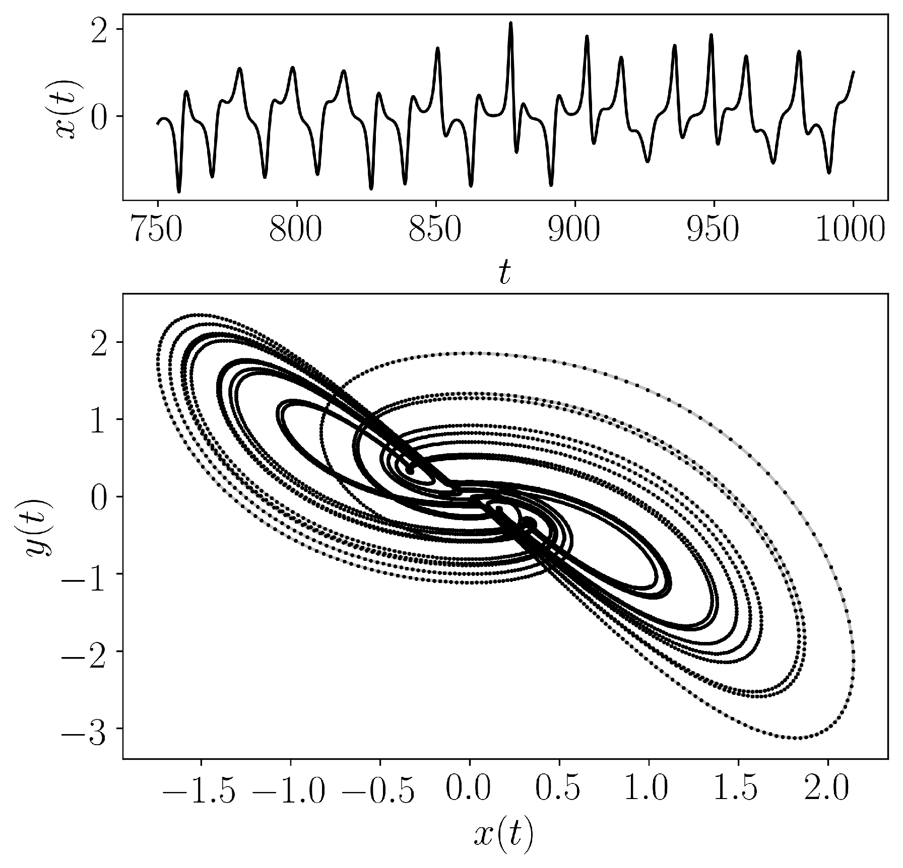
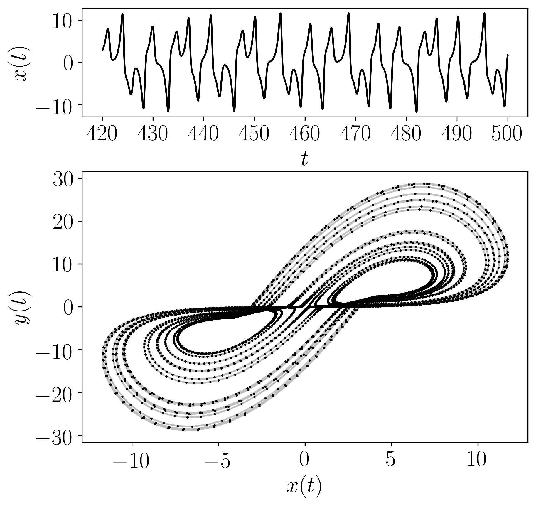
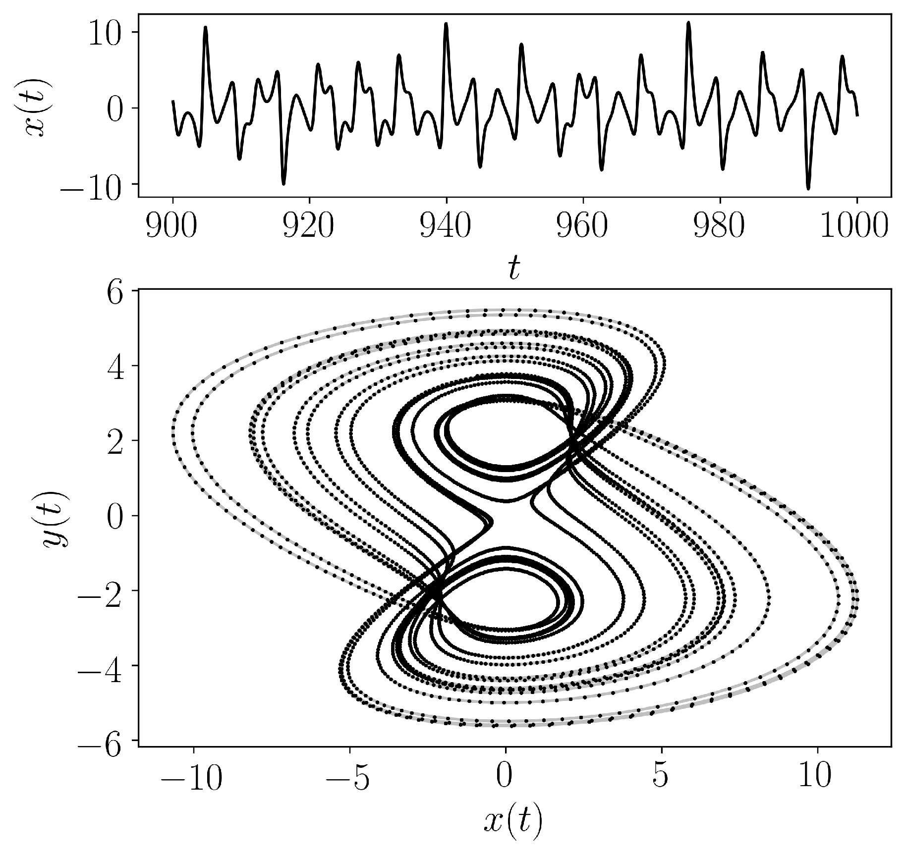
teaspoon.MakeData.DynSysLib.autonomous_dissipative_flows.chens_system(parameters=[30.0, 3.0, 28.0], dynamic_state=None, InitialConditions=[-10, 0, 37], L=500.0, fs=200, SampleSize=3000)

Chen’s System is defined [2] as

\[ \begin{align}\begin{aligned}\dot{x} &= a(y-x),\\\dot{y} &= (c-a)x-xz+cy,\\\dot{z} &= xy-bz\end{aligned}\end{align} \]

The system parameters are set to \(a = 35\), \(b = 3\), and \(c = 28\) for a chaotic response and \(a = 30\) for a periodic response. The initial conditions were set to \([x, y, z] = [-10, 0, 37]\). The system was simulated for 500 seconds at a rate of 200 Hz and the last 15 seconds were used for the chaotic response.

Parameters:

• parameters (Optional[floats]) – Array of three floats [\(a\), \(b\), \(c\)] or None if using the dynamic_state variable

• fs (Optional[float]) – Sampling rate for simulation

• SampleSize (Optional[int]) – length of sample at end of entire time series

• L (Optional[int]) – Number of iterations

• InitialConditions (Optional[floats]) – list of values for [\(x_0\), \(y_0\), \(z_0\)]

• dynamic_state (Optional[str]) – Set dynamic state as either ‘periodic’ or ‘chaotic’ if not supplying parameters.

Returns:

Array of the time indices as t and the simulation time series ts

Return type:

array

References

[2]

Liang, Xiyin. “Mechanical analysis of Chen chaotic system”. Chaos, Solitons & Fractals, 2017.

teaspoon.MakeData.DynSysLib.autonomous_dissipative_flows.hadley_circulation(parameters=[0.25, 4, 8, 1], dynamic_state=None, InitialConditions=[-10, 0, 37], L=500.0, fs=50, SampleSize=4000)

Hadley Circulation System is defined as

\[ \begin{align}\begin{aligned}\dot{x} &= -y^2 - z^2 - ax + aF,\\\dot{y} &= xy - bxz - y + G,\\\dot{z} &= bxy + xz - z\end{aligned}\end{align} \]

The system parameters are set to \(a = 0.25\), \(b = 4\), \(F = 8`and :math:`G = 1\) for a periodic response and \(a = 0.3\) for a chaotic response. The initial conditions were set to \([x, y, z] = [-10, 0, 37]\).

Parameters:

• parameters (Optional[floats]) – Array of four floats [\(a\), \(b\), \(F`\), \(G\)] or None if using the dynamic_state variable

• fs (Optional[float]) – Sampling rate for simulation

• SampleSize (Optional[int]) – length of sample at end of entire time series

• L (Optional[int]) – Number of iterations

• InitialConditions (Optional[floats]) – list of values for [\(x_0\), \(y_0\), \(z_0\)]

• dynamic_state (Optional[str]) – Set dynamic state as either ‘periodic’ or ‘chaotic’ if not supplying parameters.

Returns:

Array of the time indices as t and the simulation time series ts

Return type:

array

teaspoon.MakeData.DynSysLib.autonomous_dissipative_flows.ACT_attractor(parameters=[2.5, 0.02, 1.5, -0.07], dynamic_state=None, InitialConditions=[0.5, 0, 0], L=500.0, fs=50, SampleSize=4000)

ACT Attractor is defined [3] as

\[ \begin{align}\begin{aligned}\dot{x} &= \alpha(x-y),\\\dot{y} &= -4\alpha y + xz + \mu x^3,\\\dot{z} &= -\delta \alpha z + xy + \beta z^2\end{aligned}\end{align} \]

The system parameters are set to \(\alpha = 2.5\), \(\mu = 0.02\), \(\delta = 1.5`and :math:\)beta = -0.07` for a periodic response and \(a = 2.0\) for a chaotic response. The initial conditions were set to \([x, y, z] = [0.5, 0, 0]\).

Parameters:

• parameters (Optional[floats]) – Array of four floats [\(\alpha\), \(\mu\), \(\delta`\), \(\beta\)] or None if using the dynamic_state variable

• fs (Optional[float]) – Sampling rate for simulation

• SampleSize (Optional[int]) – length of sample at end of entire time series

• L (Optional[int]) – Number of iterations

• InitialConditions (Optional[floats]) – list of values for [\(x_0\), \(y_0\), \(z_0\)]

• dynamic_state (Optional[str]) – Set dynamic state as either ‘periodic’ or ‘chaotic’ if not supplying parameters.

Returns:

Array of the time indices as t and the simulation time series ts

Return type:

array

References

[3]

1. Arneodo, P. Coullet, and C. Tresser. Possible new strange attractors with spiral structure. Communications in Mathematical Physics, 79(4):573-579, dec 1981.

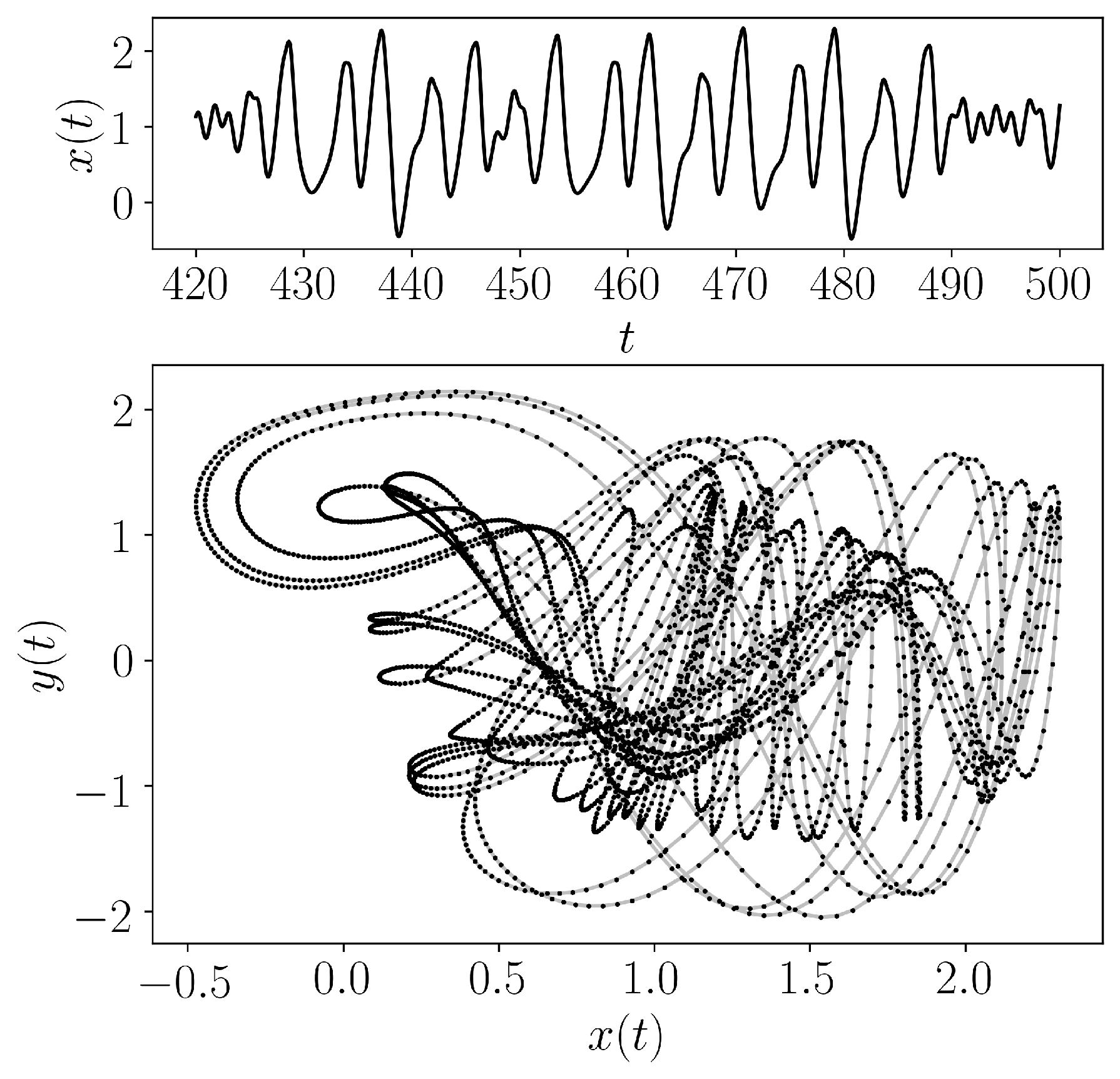
teaspoon.MakeData.DynSysLib.autonomous_dissipative_flows.rabinovich_frabrikant_attractor(parameters=[1.16, 0.87], dynamic_state=None, InitialConditions=[-1, 0, 0.5], L=500.0, fs=30, SampleSize=3000)

Rabinovich-Frabrikant Attractor is defined [4] as

\[ \begin{align}\begin{aligned}\dot{x} &= y(z - 1 + x^2) + \alpha x,\\\dot{y} &= x(3z + 1 - x^2) + \alpha y,\\\dot{z} &= -2z(\gamma + xy)\end{aligned}\end{align} \]

The system parameters are set to \(\alpha = 1.16\) and \(\gamma = 0.87\) for a periodic response and \(\alpha = 1.13\) for a chaotic response. The initial conditions were set to \([x, y, z] = [-1, 0, 0.5]\).

Parameters:

• parameters (Optional[floats]) – Array of two floats [\(\alpha\), \(\gamma\)] or None if using the dynamic_state variable

• fs (Optional[float]) – Sampling rate for simulation

• SampleSize (Optional[int]) – length of sample at end of entire time series

• L (Optional[int]) – Number of iterations

• InitialConditions (Optional[floats]) – list of values for [\(x_0\), \(y_0\), \(z_0\)]

• dynamic_state (Optional[str]) – Set dynamic state as either ‘periodic’ or ‘chaotic’ if not supplying parameters.

Returns:

Array of the time indices as t and the simulation time series ts

Return type:

array

References

[4]

Marius-F. Danca. Hidden transient chaotic attractors of rabinovich-fabrikant system. Nonlinear Dynamics, 86(2):1263-1270, jul 2016.

teaspoon.MakeData.DynSysLib.autonomous_dissipative_flows.linear_feedback_rigid_body_motion_system(parameters=[5.3, -10, -3.8], dynamic_state=None, InitialConditions=[0.2, 0.2, 0.2], L=500.0, fs=100, SampleSize=3000)

Linear Feedback Rigid Body Motion System is defined [5] as

\[ \begin{align}\begin{aligned}\dot{x} &= yx,\\\dot{y} &= xz + by,\\\dot{z} &= \frac{1}{3}xy + cz\end{aligned}\end{align} \]

The system parameters are set to \(a = 5.3\), \(b = -10\), \(c = -3.8\) for a periodic response and \(a = 5\) for a chaotic response. The initial conditions were set to \([x, y, z] = [0.2, 0.2, 0.2]\).

Parameters:

• parameters (Optional[floats]) – Array of three floats [\(a\), \(b\), \(c\)] or None if using the dynamic_state variable

• fs (Optional[float]) – Sampling rate for simulation

• SampleSize (Optional[int]) – length of sample at end of entire time series

• L (Optional[int]) – Number of iterations

• InitialConditions (Optional[floats]) – list of values for [\(x_0\), \(y_0\), \(z_0\)]

• dynamic_state (Optional[str]) – Set dynamic state as either ‘periodic’ or ‘chaotic’ if not supplying parameters.

Returns:

Array of the time indices as t and the simulation time series ts

Return type:

array

References

[5]

Hsien-Keng Chen and Ching-I Lee. Anti-control of chaos in rigid body motion. Chaos, Solitons & Fractals, 21(4):957-965, aug 2004.

teaspoon.MakeData.DynSysLib.autonomous_dissipative_flows.moore_spiegel_oscillator(parameters=[7.8, 20], dynamic_state=None, InitialConditions=[0.2, 0.2, 0.2], L=500.0, fs=100, SampleSize=5000)

The Moore-Spiegel Oscillator is defined [6] as

\[ \begin{align}\begin{aligned}\dot{x} &= y,\\\dot{y} &= z,\\\dot{z} &= -z - (T - R + Rx^2)y - Tx\end{aligned}\end{align} \]

The system parameters are set to \(T = 7.8\), \(R = 20\) for a periodic response and \(T = 7\) for a chaotic response. The initial conditions were set to \([x, y, z] = [0.2, 0.2, 0.2]\).

Parameters:

• parameters (Optional[floats]) – Array of two floats [\(T\), \(R\)] or None if using the dynamic_state variable

• fs (Optional[float]) – Sampling rate for simulation

• SampleSize (Optional[int]) – length of sample at end of entire time series

• L (Optional[int]) – Number of iterations

• InitialConditions (Optional[floats]) – list of values for [\(x_0\), \(y_0\), \(z_0\)]

• dynamic_state (Optional[str]) – Set dynamic state as either ‘periodic’ or ‘chaotic’ if not supplying parameters.

Returns:

Array of the time indices as t and the simulation time series ts

Return type:

array

References

[6]

14. 10. Balmforth and R. V. Craster. Synchronizing moore and spiegel. Chaos: An Interdisciplinary Journal of Nonlinear Science, 7(4):738-752, dec 1997.

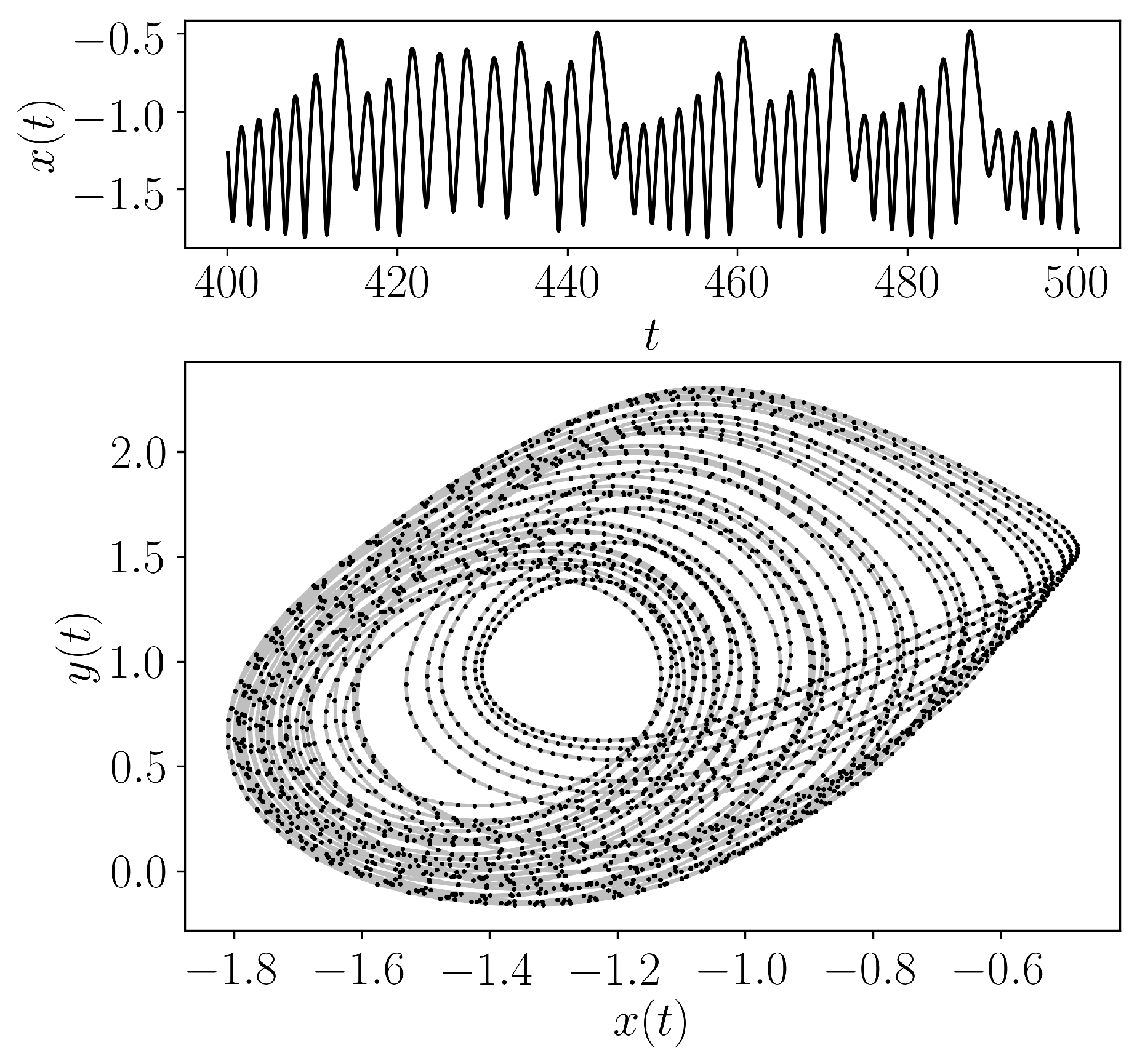
teaspoon.MakeData.DynSysLib.autonomous_dissipative_flows.thomas_cyclically_symmetric_attractor(parameters=[0.17], dynamic_state=None, InitialConditions=[0.1, 0, 0], L=1000.0, fs=10, SampleSize=5000)

The Thomas Cyclically Symmetric Attractor is defined [7] as

\[ \begin{align}\begin{aligned}\dot{x} &= -bx + \sin{y},\\\dot{y} &= -by + \sin{z},\\\dot{z} &= -bz + \sin{x}\end{aligned}\end{align} \]

The system parameters are set to \(b = 0.17\) for a periodic response and \(b = 0.18\) for a chaotic response. The initial conditions were set to \([x, y, z] = [0.1, 0, 0]\).

Parameters:

• parameters (Optional[floats]) – Array of one float [\(b\)] or None if using the dynamic_state variable

• fs (Optional[float]) – Sampling rate for simulation

• SampleSize (Optional[int]) – length of sample at end of entire time series

• L (Optional[int]) – Number of iterations

• InitialConditions (Optional[floats]) – list of values for [\(x_0\), \(y_0\), \(z_0\)]

• dynamic_state (Optional[str]) – Set dynamic state as either ‘periodic’ or ‘chaotic’ if not supplying parameters.

Returns:

Array of the time indices as t and the simulation time series ts

Return type:

array

References

[7]

18. Thomas. Deterministic chaos seen in terms of feedback circuits: Analysis, synthesis, ”labyrinth chaos”. International Journal of Bifurcation and Chaos, 9:1889-1905, 1999.

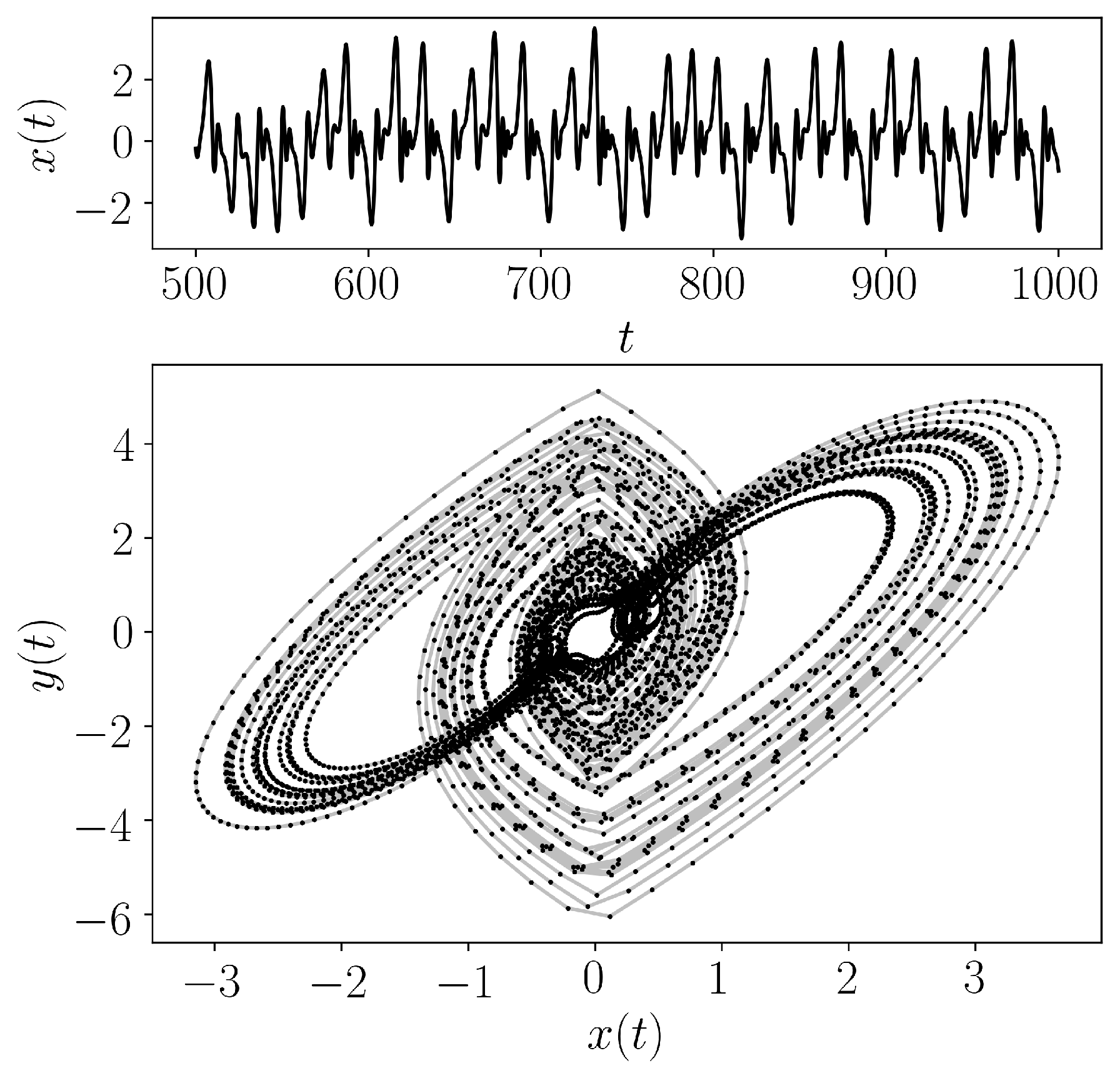
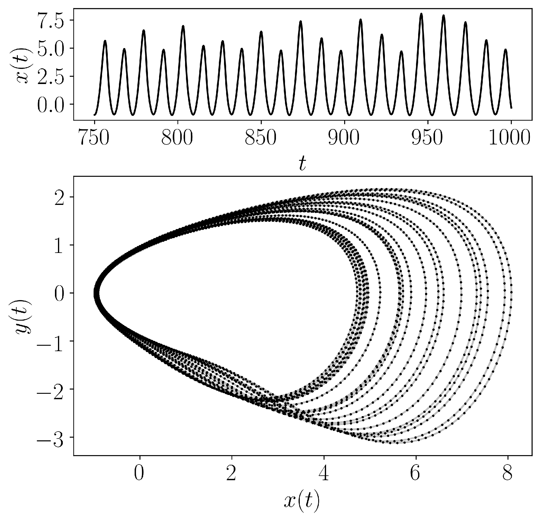
teaspoon.MakeData.DynSysLib.autonomous_dissipative_flows.halvorsens_cyclically_symmetric_attractor(parameters=[1.85, 4, 4], dynamic_state=None, InitialConditions=[-5, 0, 0], L=200.0, fs=200, SampleSize=5000)

The Halvorsens Cyclically Symmetric Attractor is defined as

\[ \begin{align}\begin{aligned}\dot{x} &= -ax - by - cz - y^2,\\\dot{y} &= -ay - bz - cz - z^2,\\\dot{z} &= -az - bx - cy - x^2\end{aligned}\end{align} \]

The system parameters are set to \(a = 1.85\), \(b = 4\), \(c = 4\) for a periodic response and \(a = 1.45\) for a chaotic response. The initial conditions were set to \([x, y, z] = [-5, 0, 0]\).

Parameters:

• parameters (Optional[floats]) – Array of three floats [\(a\), \(b\), \(c\)] or None if using the dynamic_state variable

• fs (Optional[float]) – Sampling rate for simulation

• SampleSize (Optional[int]) – length of sample at end of entire time series

• L (Optional[int]) – Number of iterations

• InitialConditions (Optional[floats]) – list of values for [\(x_0\), \(y_0\), \(z_0\)]

• dynamic_state (Optional[str]) – Set dynamic state as either ‘periodic’ or ‘chaotic’ if not supplying parameters.

Returns:

Array of the time indices as t and the simulation time series ts

Return type:

array

teaspoon.MakeData.DynSysLib.autonomous_dissipative_flows.burke_shaw_attractor(parameters=[12.0, 4.0], dynamic_state=None, InitialConditions=[0.6, 0.0, 0.0], L=500.0, fs=200, SampleSize=5000)

The Burke-Shaw Attractor is defined [8] as

\[ \begin{align}\begin{aligned}\dot{x} &= s(x+y),\\\dot{y} &= -y - sxz,\\\dot{z} &= sxy + V\end{aligned}\end{align} \]

The system parameters are set to \(s = 12\), \(V = 4\), and \(c = 28\) for a periodic response and \(s = 10\) for a chaotic response. The initial conditions were set to \([x, y, z] = [0.6,0.0,0.0]\). The system was simulated for 500 seconds at a rate of 200 Hz and the last 25 seconds were used for the chaotic response.

Parameters:

• parameters (Optional[floats]) – Array of two floats [\(s\), \(V\)] or None if using the dynamic_state variable

• fs (Optional[float]) – Sampling rate for simulation

• SampleSize (Optional[int]) – length of sample at end of entire time series

• L (Optional[int]) – Number of iterations

• InitialConditions (Optional[floats]) – list of values for [\(x_0\), \(y_0\), \(z_0\)]

• dynamic_state (Optional[str]) – Set dynamic state as either ‘periodic’ or ‘chaotic’ if not supplying parameters.

Returns:

Array of the time indices as t and the simulation time series ts

Return type:

array

References

[8]

Shaw, Robert. “Strange attractors, chaotic behavior, and information flow”. Zeitschrift für Naturforschung, 1981.

teaspoon.MakeData.DynSysLib.autonomous_dissipative_flows.rucklidge_attractor(parameters=[1.1, 6.7], dynamic_state=None, InitialConditions=[1.0, 0.0, 4.5], L=1000.0, fs=50, SampleSize=5000)

The Rucklidge Attractor is defined [9] as

\[ \begin{align}\begin{aligned}\dot{x} &= -kx + \lambda y - yz,\\\dot{y} &= x,\\\dot{z} &= -z + y^2\end{aligned}\end{align} \]

The system parameters are set to \(k = 1.1\), \(\lambda = 6.7\) for a periodic response and \(k = 1.6\) for a chaotic response. The initial conditions were set to \([x, y, z] = [1.0,0.0,4.5]\). The system was simulated for 1000 seconds at a rate of 50 Hz and the last 100 seconds were used for the chaotic response.

Parameters:

• parameters (Optional[floats]) – Array of two floats [\(k\), \(\lambda\)] or None if using the dynamic_state variable

• fs (Optional[float]) – Sampling rate for simulation

• SampleSize (Optional[int]) – length of sample at end of entire time series

• L (Optional[int]) – Number of iterations

• InitialConditions (Optional[floats]) – list of values for [\(x_0\), \(y_0\), \(z_0\)]

• dynamic_state (Optional[str]) – Set dynamic state as either ‘periodic’ or ‘chaotic’ if not supplying parameters.

Returns:

Array of the time indices as t and the simulation time series ts

Return type:

array

References

[9]

Chandrasekaran, Ramanathan. “A new chaotic attractor from Rucklidge system and its application in secured communication using OFDM”. 11th International Conference on Intelligent Systems and Control (ISCO), 2017.

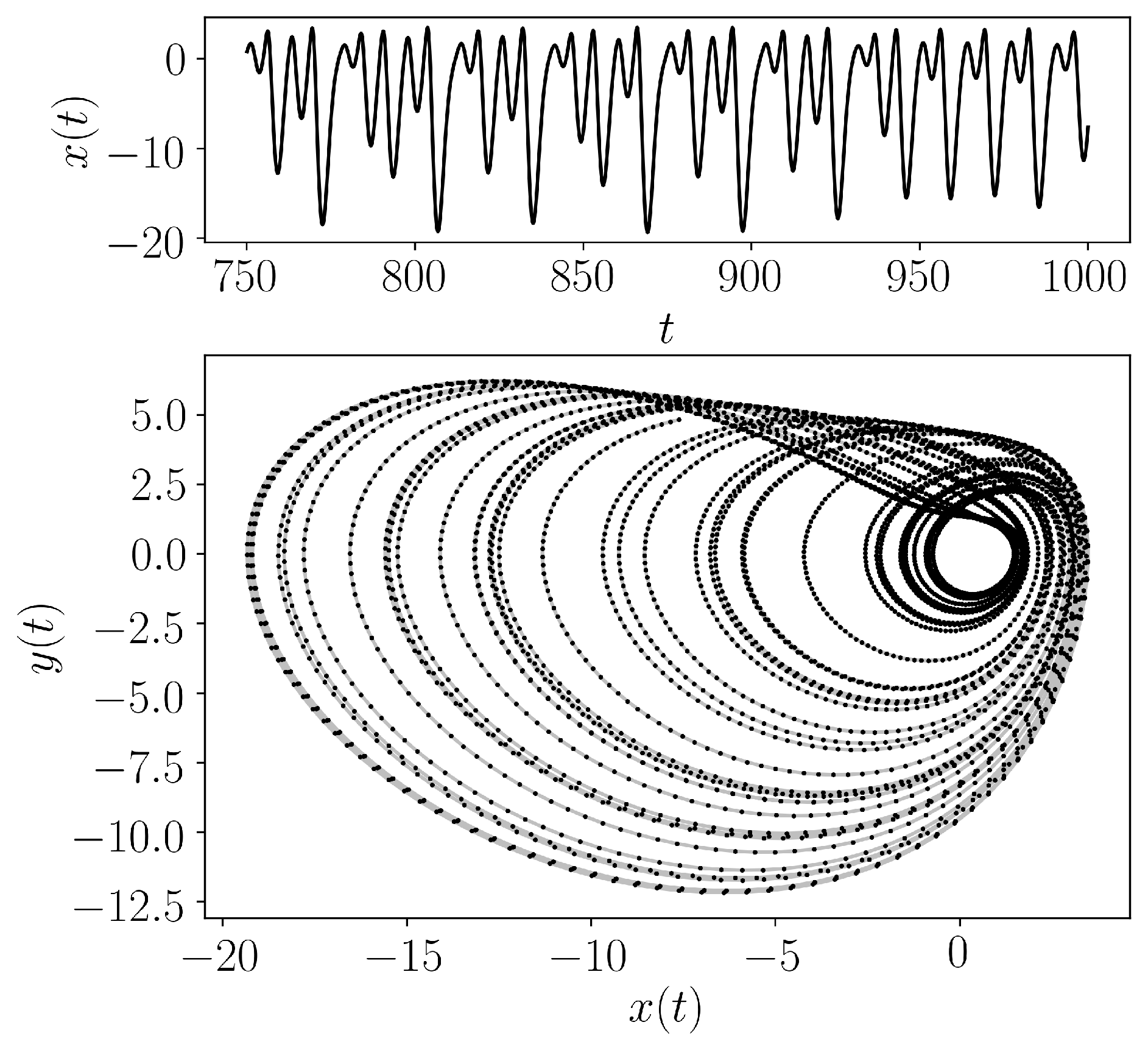
teaspoon.MakeData.DynSysLib.autonomous_dissipative_flows.WINDMI(parameters=[0.9, 2.5], dynamic_state=None, InitialConditions=[1.0, 0.0, 4.5], L=1000.0, fs=20, SampleSize=5000)

The WINDMI Attractor is defined [10] as

\[ \begin{align}\begin{aligned}\dot{x} &= y,\\\dot{y} &= z,\\\dot{z} &= -az - y + b - e^x\end{aligned}\end{align} \]

The system parameters are set to \(a = 0.9\), \(b = 2.5\) for a periodic response and \(a = 0.8\) for a chaotic response. The initial conditions were set to \([x, y, z] = [1.0,0.0,4.5]\). The system was simulated for 1000 seconds at a rate of 20 Hz and the last 250 seconds were used for the chaotic response.

Parameters:

• parameters (Optional[floats]) – Array of two floats [\(a\), \(b\)] or None if using the dynamic_state variable

• fs (Optional[float]) – Sampling rate for simulation

• SampleSize (Optional[int]) – length of sample at end of entire time series

• L (Optional[int]) – Number of iterations

• InitialConditions (Optional[floats]) – list of values for [\(x_0\), \(y_0\), \(z_0\)]

• dynamic_state (Optional[str]) – Set dynamic state as either ‘periodic’ or ‘chaotic’ if not supplying parameters.

Returns:

Array of the time indices as t and the simulation time series ts

Return type:

array

References

[10]

Vaidyanathan, S. “Adaptive backstepping controller design for the anti - synchronization of identical WINDMI chaotic systems with unknown parameters and its SPICE implementation”. Journal of Engineering Science and Technology Review, 2015.

teaspoon.MakeData.DynSysLib.autonomous_dissipative_flows.simplest_quadratic_chaotic_flow(parameters=[2.017, 1.0], dynamic_state=None, InitialConditions=[-0.9, 0.0, 0.5], L=1000.0, fs=20, SampleSize=5000)

The Simplest Quadratic Chaotic Flow is defined [11] as

\[ \begin{align}\begin{aligned}\dot{x} &= y,\\\dot{y} &= z,\\\dot{z} &= -az - by^2 - x\end{aligned}\end{align} \]

The system parameters are set to \(a = 2.017\), \(b = 1.0\) for a chaotic response we could not find any periodic response near this value. The initial conditions were set to \([x, y, z] = [-0.9,0.0,0.5]\). The system was simulated for 1000 seconds at a rate of 20 Hz and the last 250 seconds were used for the chaotic response.

Parameters:

• parameters (Optional[floats]) – Array of two floats [\(a\), \(b\)] or None if using the dynamic_state variable

• fs (Optional[float]) – Sampling rate for simulation

• SampleSize (Optional[int]) – length of sample at end of entire time series

• L (Optional[int]) – Number of iterations

• InitialConditions (Optional[floats]) – list of values for [\(x_0\), \(y_0\), \(z_0\)]

• dynamic_state (Optional[str]) – Set dynamic state as either ‘periodic’ or ‘chaotic’ if not supplying parameters.

Returns:

Array of the time indices as t and the simulation time series ts

Return type:

array

References

[11]

Sprott, J.C. “Simplest dissipative chaotic flow”. Physics Letters A, 1997.

teaspoon.MakeData.DynSysLib.autonomous_dissipative_flows.simplest_cubic_chaotic_flow(parameters=[2.11, 2.5], dynamic_state=None, InitialConditions=[0.0, 0.96, 0.0], L=1000.0, fs=20, SampleSize=5000)

The Simplest Cubic Chaotic Flow is defined [12] as

\[ \begin{align}\begin{aligned}\dot{x} &= y,\\\dot{y} &= z,\\\dot{z} &= -az - xy^2 - x\end{aligned}\end{align} \]

The system parameters are set to \(a = 2.11\), \(b = 2.5\) for a periodic response and \(a = 2.05\) for chaotic. The initial conditions were set to \([x, y, z] = [0.0,0.96,0.0]\). The system was simulated for 1000 seconds at a rate of 20 Hz and the last 250 seconds were used for the chaotic response.

Parameters:

• parameters (Optional[floats]) – Array of two floats [\(a\), \(b\)] or None if using the dynamic_state variable

• fs (Optional[float]) – Sampling rate for simulation

• SampleSize (Optional[int]) – length of sample at end of entire time series

• L (Optional[int]) – Number of iterations

• InitialConditions (Optional[floats]) – list of values for [\(x_0\), \(y_0\), \(z_0\)]

• dynamic_state (Optional[str]) – Set dynamic state as either ‘periodic’ or ‘chaotic’ if not supplying parameters.

Returns:

Array of the time indices as t and the simulation time series ts

Return type:

array

References

[12]

Malasomam, J.-M. “What is the simplest dissipative chaotic jerk equation which is parity invariant?” Physics Letters A, 2000.

teaspoon.MakeData.DynSysLib.autonomous_dissipative_flows.simplest_piecewise_linear_chaotic_flow(parameters=[0.7], dynamic_state=None, InitialConditions=[0.0, -0.7, 0.0], L=1000.0, fs=40, SampleSize=5000)

The Simplest Piecewise-Linear Chaotic Flow is defined [13] as

\[ \begin{align}\begin{aligned}\dot{x} &= y,\\\dot{y} &= z,\\\dot{z} &= -az - y + |x| - 1\end{aligned}\end{align} \]

The system parameter is set to \(a = 0.7\) for a periodic response and \(a = 0.6\) for chaotic. The initial conditions were set to \([x, y, z] = [0.0,-0.7,0.0]\). The system was simulated for 1000 seconds at a rate of 20 Hz and the last 250 seconds were used for the chaotic response.

Parameters:

• parameters (Optional[floats]) – Array of one float [\(a\)] or None if using the dynamic_state variable

• fs (Optional[float]) – Sampling rate for simulation

• SampleSize (Optional[int]) – length of sample at end of entire time series

• L (Optional[int]) – Number of iterations

• InitialConditions (Optional[floats]) – list of values for [\(x_0\), \(y_0\), \(z_0\)]

• dynamic_state (Optional[str]) – Set dynamic state as either ‘periodic’ or ‘chaotic’ if not supplying parameters.

Returns:

Array of the time indices as t and the simulation time series ts

Return type:

array

References

[13]

TAO YANG. “PIECEWISE-LINEAR CHAOTIC SYSTEMS WITH a SINGLE EQUILIBRIUM POINT” International Journal of Bifurcation and Chaos, 2000.

teaspoon.MakeData.DynSysLib.autonomous_dissipative_flows.double_scroll(parameters=[1.0], dynamic_state=None, InitialConditions=[0.01, 0.01, 0.0], L=1000.0, fs=20, SampleSize=5000)

The Double Scroll Attractor is defined [14] as

\[ \begin{align}\begin{aligned}\dot{x} &= y,\\\dot{y} &= z,\\\dot{z} &= -a(x + y + z - \text{sgn}(x))\end{aligned}\end{align} \]

The system parameter is set to \(a = 1.0\) for a periodic response and \(a = 0.8\) for chaotic. The initial conditions were set to \([x, y, z] = [0.01,0.01,0.0]\). The system was simulated for 1000 seconds at a rate of 20 Hz and the last 250 seconds were used for the chaotic response.

Parameters:

• parameters (Optional[floats]) – Array of one float [\(a\)] or None if using the dynamic_state variable

• fs (Optional[float]) – Sampling rate for simulation

• SampleSize (Optional[int]) – length of sample at end of entire time series

• L (Optional[int]) – Number of iterations

• InitialConditions (Optional[floats]) – list of values for [\(x_0\), \(y_0\), \(z_0\)]

• dynamic_state (Optional[str]) – Set dynamic state as either ‘periodic’ or ‘chaotic’ if not supplying parameters.

Returns:

Array of the time indices as t and the simulation time series ts

Return type:

array

References

[14]

A.S Elwakil “Chua’s circuit decomposition: a systematic design approach for chaotic oscillators” Journal of the Franklin Institute, 2000.

2.1.2.2.2. Meta Function

This function is for being able to input into the original teaspoon.MakeData.DynSysLib.DynamicSystems function with default parameters.

teaspoon.MakeData.DynSysLib.autonomous_dissipative_flows.autonomous_dissipative_flows(system, dynamic_state=None, L=None, fs=None, SampleSize=None, parameters=None, InitialConditions=None)