2.1.2.3. Driven Dissipative Flows
2.1.2.3.1. Main Functions
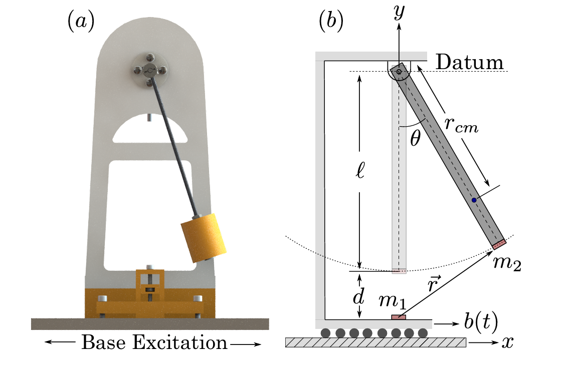
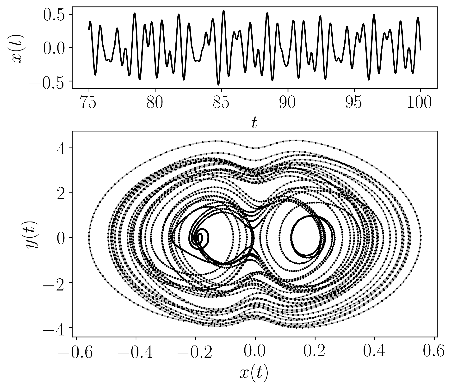
- teaspoon.MakeData.DynSysLib.driven_dissipative_flows.base_excited_magnetic_pendulum(parameters=[0.1038, 0.208, 9.81, 0.18775, 1.919e-05, 0.022, 9.42477796076938, 0.003, 1.2, 0.032, 1.257e-06], fs=200, SampleSize=5000, L=100.0, dynamic_state=None, InitialConditions=[0.0, 0.0])[source]
This is a simple pendulum with a magnet at its base. See Myers & Khasawneh [1]. The system was simulated for 100 seconds at a rate of 200 Hz and the last 25 seconds were used for the chaotic response as shown in the figure below.
- Parameters:
L (Optional[int]) – Number of iterations.
fs (Optional[int]) – sampling rate for simulation.
SampleSize (Optional[int]) – length of sample at end of entire time series
parameters (Optional[floats]) – list of values for [m, l, g, r_cm, I_o, A, w, c, q, d, mu] or None if using the dynamic_state variable
InitialConditions (Optional[floats]) – list of values for [\(x_0\), \(y_0\)]
dynamic_state (Optional[str]) – Set dynamic state as either ‘periodic’ or ‘chaotic’ if not supplying parameters.
Returns
array – Array of the time indices as t and the simulation time series ts
References
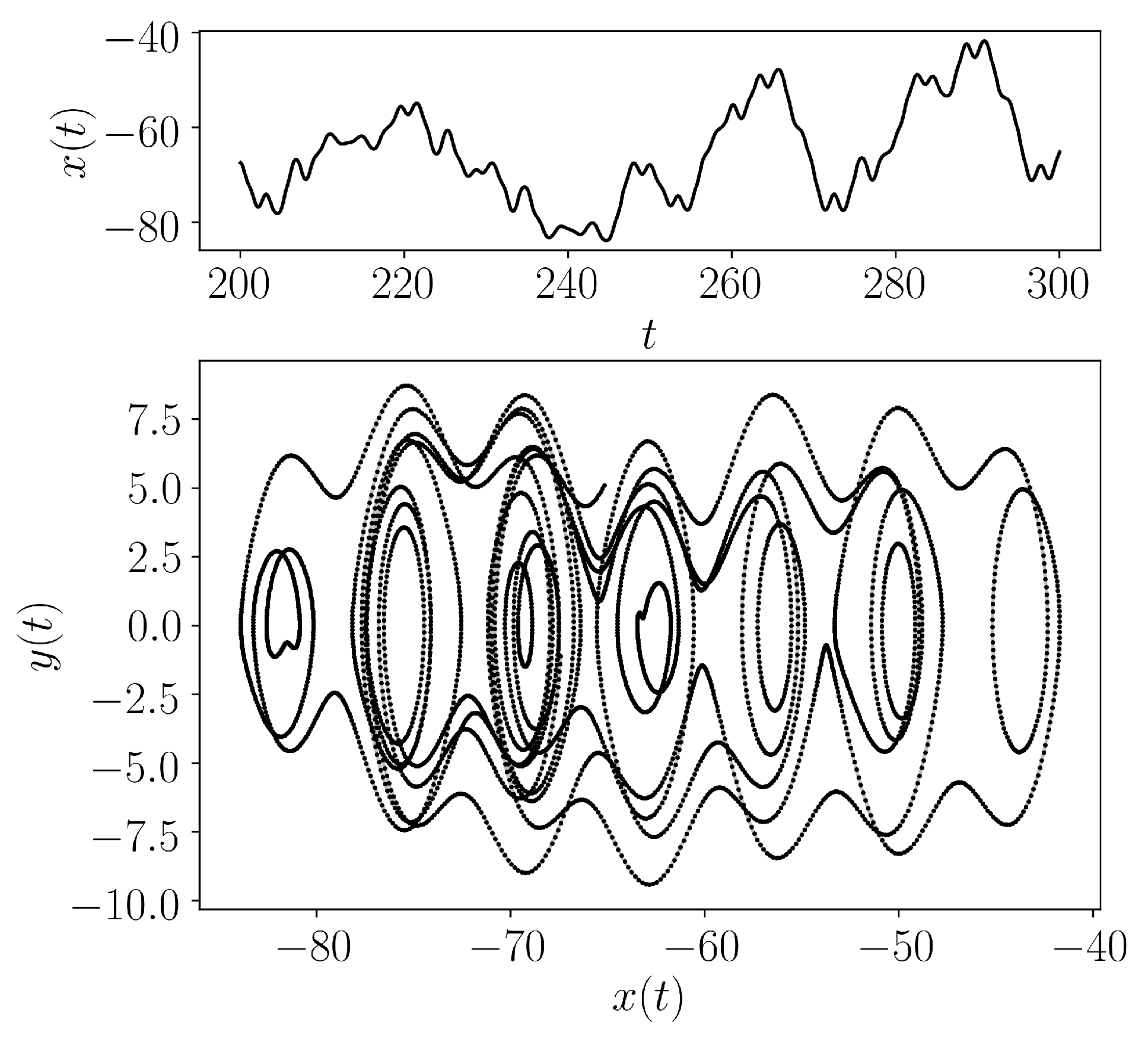
- teaspoon.MakeData.DynSysLib.driven_dissipative_flows.driven_pendulum(fs=50, SampleSize=5000, L=300, parameters=[1, 9.81, 1, 0.1, 5, 1], InitialConditions=[0, 0], dynamic_state=None)[source]
The point mass, driven simple pendulum with viscous damping is described as
\[ \begin{align}\begin{aligned}\dot{\theta} = \omega,\\\dot{\omega} = -\frac{g}{l}\sin{\theta} + \frac{A}{ml^2}\sin{\omega_m t} - c\omega\end{aligned}\end{align} \]where we chose the parameters \(g = 9.81\) for gravitational constant, \(l = 1\) for the length of pendulum arm, \(m = 1\) for the point mass, \(A = 5\) for the amplitude of force, and \(\omega = 1\) for driving force (periodic) and \(\omega = 2\) for a chaotic state. The system was simulated for 300 seconds at a rate of 50 Hz and the last 100 seconds were used for the chaotic response as shown in the figure below.
- Parameters:
L (Optional[int]) – Number of iterations.
fs (Optional[int]) – sampling rate for simulation.
SampleSize (Optional[int]) – length of sample at end of entire time series
parameters (Optional[floats]) – list of values for [m, g, l, c, A, w] or None if using the dynamic_state variable
InitialConditions (Optional[floats]) – list of values for [\(\theta_0\), \(\omega_0\)]
dynamic_state (Optional[str]) – Set dynamic state as either ‘periodic’ or ‘chaotic’ if not supplying parameters.
- Returns:
Array of the time indices as t and the simulation time series ts
- Return type:
array
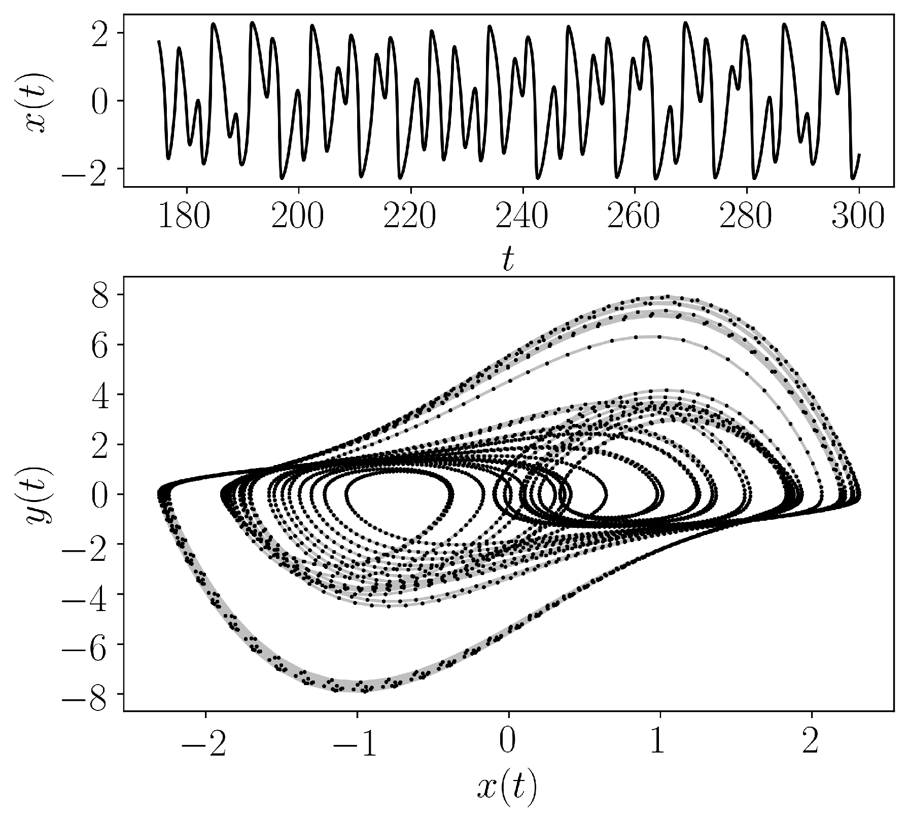
- teaspoon.MakeData.DynSysLib.driven_dissipative_flows.driven_van_der_pol_oscillator(fs=40, SampleSize=5000, L=300, parameters=[2.9, 5, 1.788], InitialConditions=[-1.9, 0], dynamic_state=None)[source]
The Driven Van der Pol Oscillator is defined as
\[ \begin{align}\begin{aligned}\dot{x} = y,\\\dot{y} = -x + b(1 - x^2)y + A\sin{\omega t}\end{aligned}\end{align} \]where we chose the parameters \((x_0. y_0) = (-1.0, 0.0)\) for initial conditions, \(A = 5\), \(\omega = 1.788\), \(b = 2.9\) (periodic) and \(b = 3.0\) (chaotic).
- Parameters:
L (Optional[int]) – Number of iterations.
fs (Optional[int]) – sampling rate for simulation.
SampleSize (Optional[int]) – length of sample at end of entire time series
parameters (Optional[floats]) – list of values for [b, A, \(\omega\)] or None if using the dynamic_state variable
InitialConditions (Optional[floats]) – list of values for [\(x_0\), \(y_0\)]
dynamic_state (Optional[str]) – Set dynamic state as either ‘periodic’ or ‘chaotic’ if not supplying parameters.
- Returns:
Array of the time indices as t and the simulation time series ts
- Return type:
array
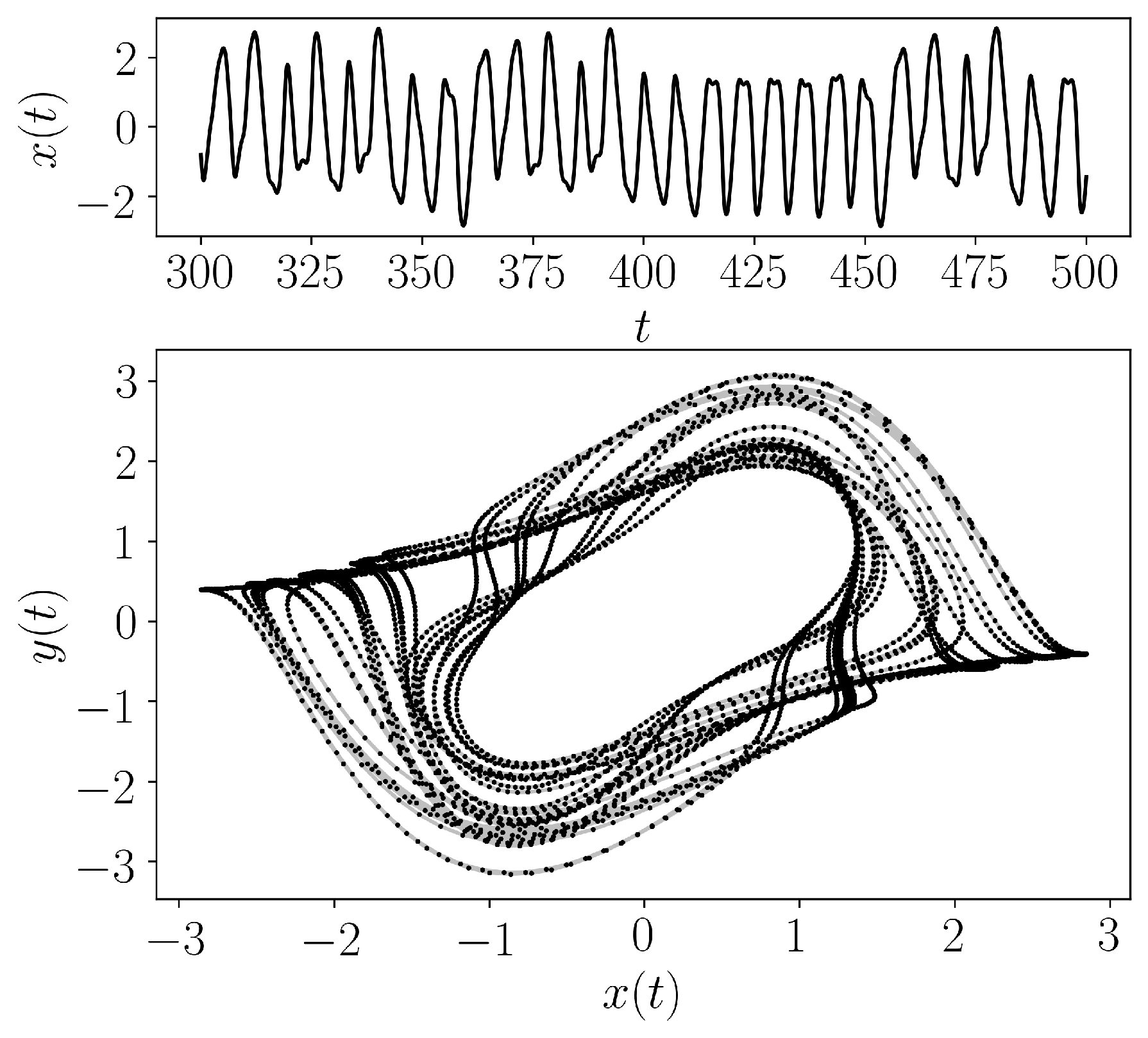
- teaspoon.MakeData.DynSysLib.driven_dissipative_flows.shaw_van_der_pol_oscillator(fs=25, SampleSize=5000, L=500.0, parameters=[1, 5, 1.4], InitialConditions=[1.3, 0], dynamic_state=None)[source]
The Shaw Van der Pol Oscillator is defined as
\[ \begin{align}\begin{aligned}\dot{x} = y + \sin{\omega t},\\\dot{y} = -x + b(1 - x^2)y\end{aligned}\end{align} \]where we chose the parameters \((x_0. y_0) = (1.3, 0.0)\) for initial conditions, \(A = 5\), \(b = 1\), \(\omega = 1.4\) (periodic) and \(\omega = 1.8\) (chaotic).
- Parameters:
L (Optional[int]) – Number of iterations.
fs (Optional[int]) – sampling rate for simulation.
SampleSize (Optional[int]) – length of sample at end of entire time series
parameters (Optional[floats]) – list of values for [b, A, \(\omega\)] or None if using the dynamic_state variable
InitialConditions (Optional[floats]) – list of values for [\(x_0\), \(y_0\)]
dynamic_state (Optional[str]) – Set dynamic state as either ‘periodic’ or ‘chaotic’ if not supplying parameters.
- Returns:
Array of the time indices as t and the simulation time series ts
- Return type:
array
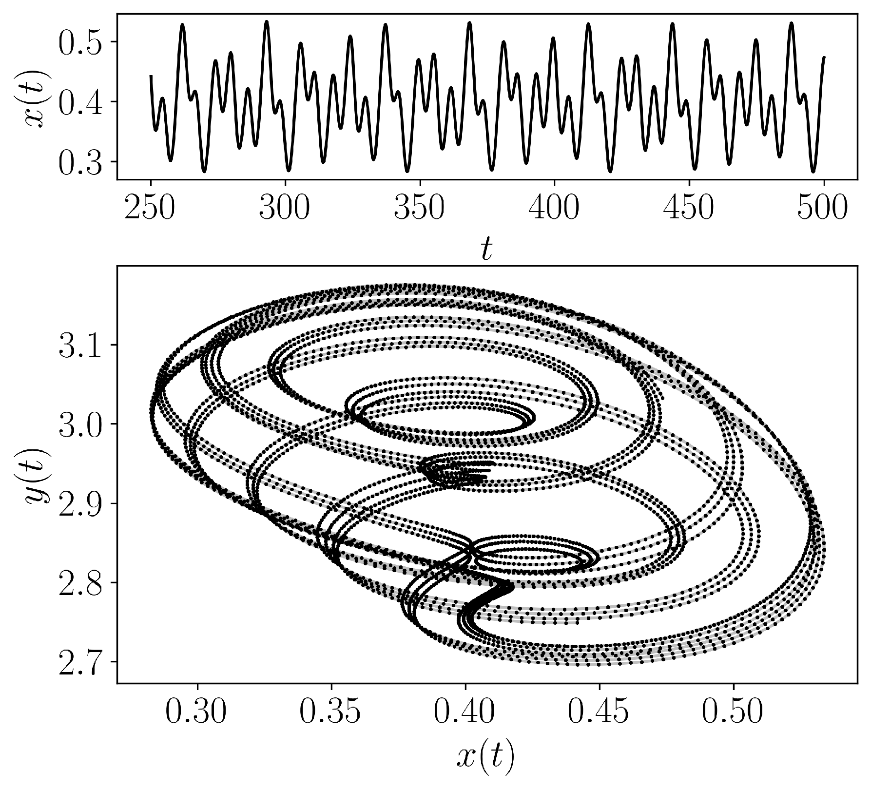
- teaspoon.MakeData.DynSysLib.driven_dissipative_flows.forced_brusselator(fs=20, SampleSize=5000, L=500.0, parameters=[0.4, 1.2, 0.05, 1.1], InitialConditions=[0.3, 2], dynamic_state=None)[source]
The Forced Brusselator is defined as
\[ \begin{align}\begin{aligned}\dot{x} = x^2y - (b+1)x + a + A\sin{\omega t},\\\dot{y} = -x^2y + bx\end{aligned}\end{align} \]where we chose the parameters \((x_0. y_0) = (0.3, 2.0)\) for initial conditions, \(a = 0.4\), \(b = 1.2\), \(A = 0.05\), \(\omega = 1.1\) (periodic) and \(\omega = 1.0\) (chaotic).
- Parameters:
L (Optional[int]) – Number of iterations.
fs (Optional[int]) – sampling rate for simulation.
SampleSize (Optional[int]) – length of sample at end of entire time series
parameters (Optional[floats]) – list of values for [a, b, A, \(\omega\)] or None if using the dynamic_state variable
InitialConditions (Optional[floats]) – list of values for [\(x_0\), \(y_0\)]
dynamic_state (Optional[str]) – Set dynamic state as either ‘periodic’ or ‘chaotic’ if not supplying parameters.
- Returns:
Array of the time indices as t and the simulation time series ts
- Return type:
array
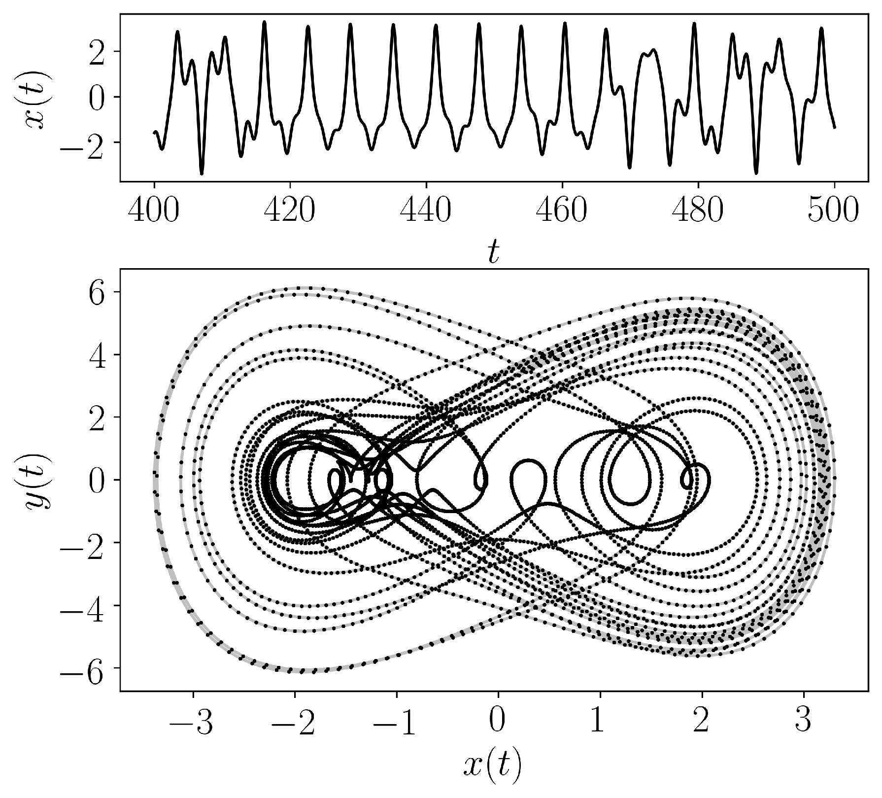
- teaspoon.MakeData.DynSysLib.driven_dissipative_flows.ueda_oscillator(fs=50, SampleSize=5000, L=500.0, parameters=[0.05, 7.5, 1.2], InitialConditions=[2.5, 0.0], dynamic_state=None)[source]
The Ueda Oscillator is defined as
\[ \begin{align}\begin{aligned}\dot{x} = y,\\\dot{y} = -x^3 - by + A\sin{\omega t}\end{aligned}\end{align} \]where we chose the parameters \((x_0. y_0) = (2.5, 0.0)\) for initial conditions, \(b = 0.05\), \(A = 7.5\), \(\omega = 1.2\) (periodic) and \(\omega = 1.0\) (chaotic).
- Parameters:
L (Optional[int]) – Number of iterations.
fs (Optional[int]) – sampling rate for simulation.
SampleSize (Optional[int]) – length of sample at end of entire time series
parameters (Optional[floats]) – list of values for [b, A, \(\omega\)] or None if using the dynamic_state variable
InitialConditions (Optional[floats]) – list of values for [\(x_0\), \(y_0\)]
dynamic_state (Optional[str]) – Set dynamic state as either ‘periodic’ or ‘chaotic’ if not supplying parameters.
- Returns:
Array of the time indices as t and the simulation time series ts
- Return type:
array
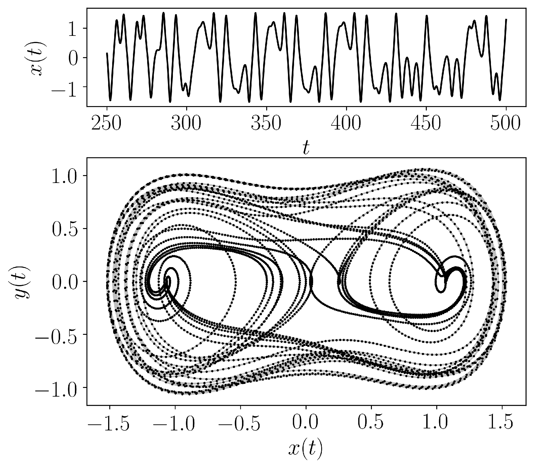
- teaspoon.MakeData.DynSysLib.driven_dissipative_flows.duffings_two_well_oscillator(fs=20, SampleSize=5000, L=500.0, parameters=[0.25, 0.4, 1.1], InitialConditions=[0.2, 0.0], dynamic_state=None)[source]
The Duffings Two-Well Oscillator is defined as
\[ \begin{align}\begin{aligned}\dot{x} = y,\\\dot{y} = -x^3 + x - by + A\sin{\omega t}\end{aligned}\end{align} \]where we chose the parameters \((x_0. y_0) = (2.5, 0.0)\) for initial conditions, \(b = 0.25\), \(A = 0.4\), \(\omega = 1.1\) (periodic) and \(\omega = 1.0\) (chaotic).
- Parameters:
L (Optional[int]) – Number of iterations.
fs (Optional[int]) – sampling rate for simulation.
SampleSize (Optional[int]) – length of sample at end of entire time series
parameters (Optional[floats]) – list of values for [b, A, \(\omega\)] or None if using the dynamic_state variable
InitialConditions (Optional[floats]) – list of values for [\(x_0\), \(y_0\)]
dynamic_state (Optional[str]) – Set dynamic state as either ‘periodic’ or ‘chaotic’ if not supplying parameters.
- Returns:
Array of the time indices as t and the simulation time series ts
- Return type:
array
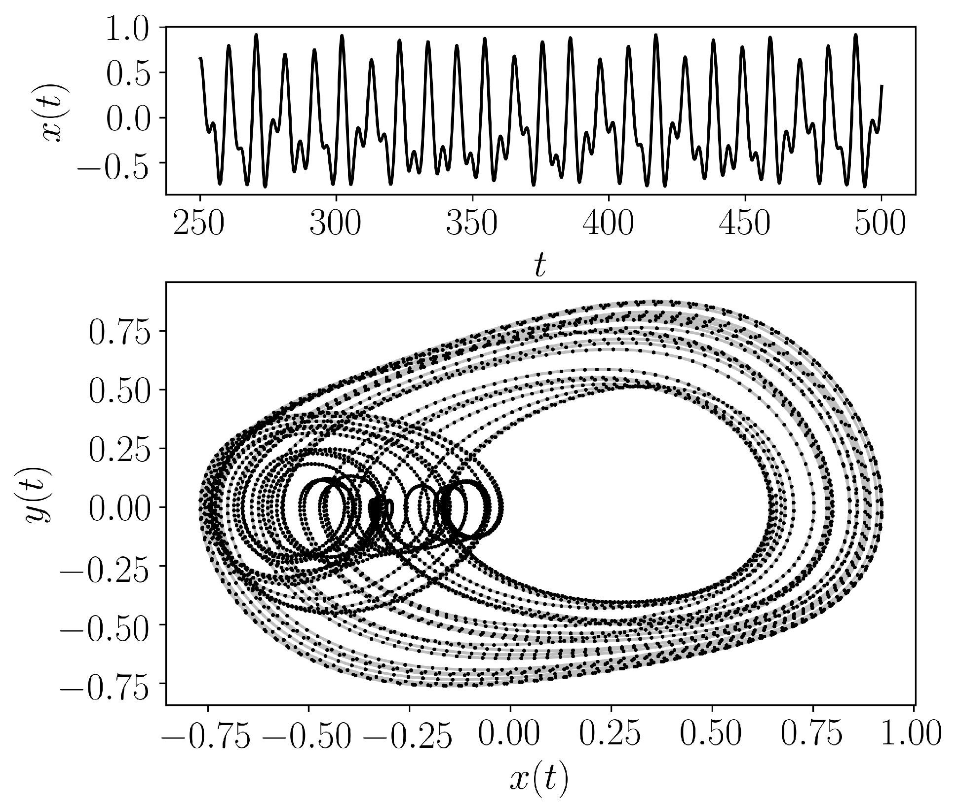
- teaspoon.MakeData.DynSysLib.driven_dissipative_flows.duffing_van_der_pol_oscillator(fs=20, SampleSize=5000, L=500.0, parameters=[0.2, 8, 0.35, 1.3], InitialConditions=[0.2, -0.2], dynamic_state=None)[source]
The Duffings Two-Well Oscillator is defined as
\[ \begin{align}\begin{aligned}\dot{x} = y,\\\dot{y} = \mu (1 - \gamma x^2)y - x^3 + A\sin{\omega t}\end{aligned}\end{align} \]where we chose the parameters \((x_0. y_0) = (0.2, 0.0)\) for initial conditions, \(\mu = 0.2\), \(\gamma = 8\), \(A = 0.35\), \(\omega = 1.3\) (periodic) and \(\omega = 1.2\) (chaotic).
- Parameters:
L (Optional[int]) – Number of iterations.
fs (Optional[int]) – sampling rate for simulation.
SampleSize (Optional[int]) – length of sample at end of entire time series
parameters (Optional[floats]) – list of values for [\(\mu\), \(\gamma\) A, \(\omega\)] or None if using the dynamic_state variable
InitialConditions (Optional[floats]) – list of values for [\(x_0\), \(y_0\)]
dynamic_state (Optional[str]) – Set dynamic state as either ‘periodic’ or ‘chaotic’ if not supplying parameters.
- Returns:
Array of the time indices as t and the simulation time series ts
- Return type:
array
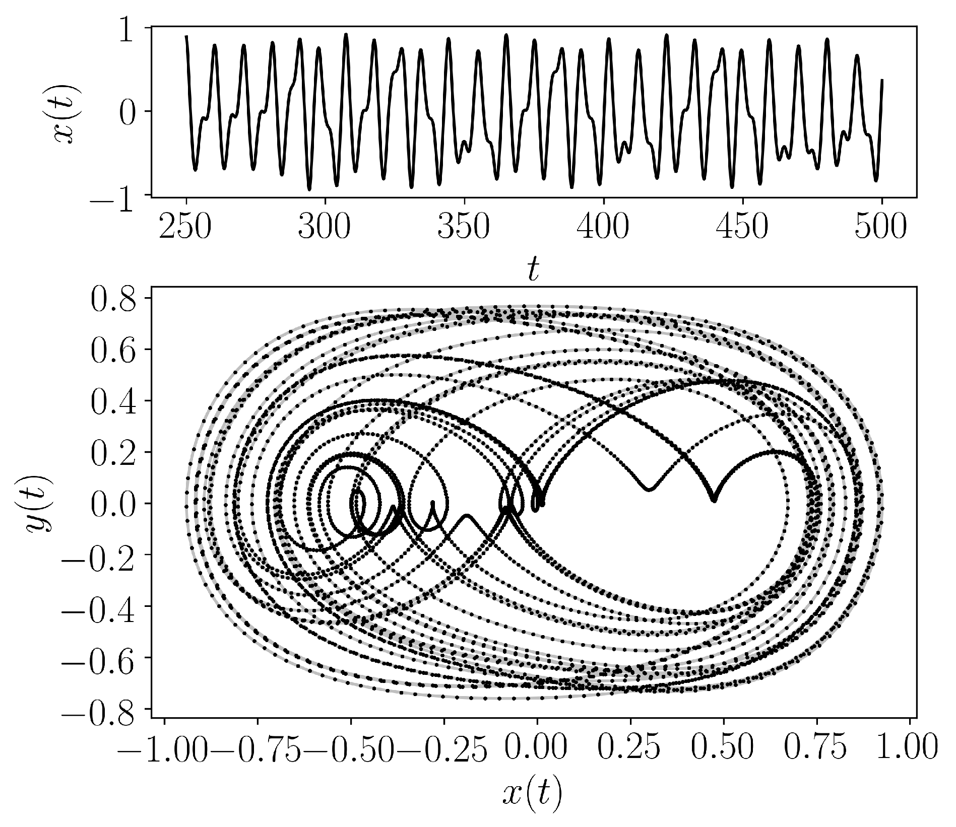
- teaspoon.MakeData.DynSysLib.driven_dissipative_flows.rayleigh_duffing_oscillator(fs=20, SampleSize=5000, L=500.0, parameters=[0.2, 4, 0.3, 1.4], InitialConditions=[0.3, 0.0], dynamic_state=None)[source]
The Rayleigh Duffing Oscillator is defined as
\[ \begin{align}\begin{aligned}\dot{x} = y,\\\dot{y} = \mu (1 - \gamma y^2)y - x^3 + A\sin{\omega t}\end{aligned}\end{align} \]where we chose the parameters \((x_0. y_0) = (0.3, 0.0)\) for initial conditions, \(\mu = 0.2\), \(\gamma = 4\), \(A = 0.3\), \(\omega = 1.4\) (periodic) and \(\omega = 1.2\) (chaotic).
- Parameters:
L (Optional[int]) – Number of iterations.
fs (Optional[int]) – sampling rate for simulation.
SampleSize (Optional[int]) – length of sample at end of entire time series
parameters (Optional[floats]) – list of values for [\(\mu\), \(\gamma\) A, \(\omega\)] or None if using the dynamic_state variable
InitialConditions (Optional[floats]) – list of values for [\(x_0\), \(y_0\)]
dynamic_state (Optional[str]) – Set dynamic state as either ‘periodic’ or ‘chaotic’ if not supplying parameters.
- Returns:
Array of the time indices as t and the simulation time series ts
- Return type:
array