2.1.2. Temporal Graph Analysis using Zigzag Persistence
This module contains code to run zigzag persistence on temporal hypergraph data. This code is based on the work performed in “Temporal Network Analysis Using Zigzag Persistence.” The general pipeline for this work is shown in the following figure.
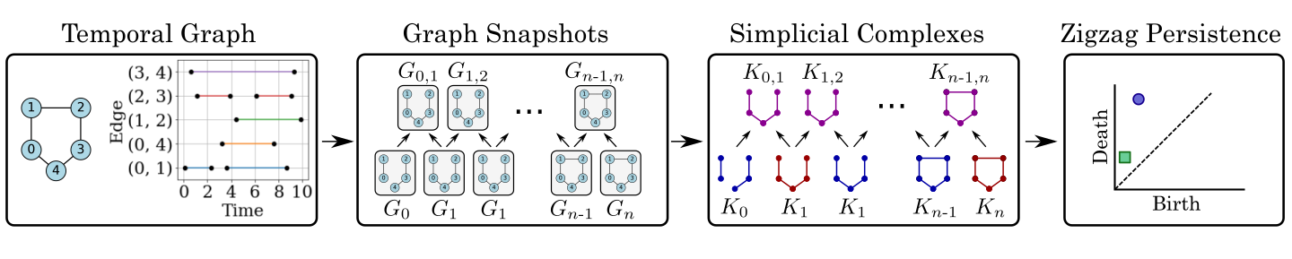
Specifically, a temporal graph is a graph whose edges are active during specified intervals. For example, conisder the edge between nodes a and b with a set of intervals associated to it. This set of intervals describes when this edge is active. An example of this is shown on the left side of the pipeline figure. Next, we generate graph snapshots from the temporal graph by using a sliding window technique. These graph snapshots are generated based on adding edges to the graph snapshot if there is an overlap between the edge’s interval and the sliding window interval. Additionally. we include union windows between sliding windows for the zigzag persistence pipeline. These union windows are formed the same except with the sliding window of the union of two temporally adjacent windows. Next, we construct simplicial complex representations for each graph and lastly apply zigzag persistence to the simplicial complex sequence.
2.1.2.1. Functions
- sporktda.TDA.TGZZ.graph_snapshots(edges, I, windows)[source]
This function gets generates graph snapshots from the temporal graph information and windows.
- Parameters:
edges (array of tuples) – edges of graph.
I (list of arrays) – list of all intervals for each edge indexed according to edge list.
windows (2xN array) – array of N intervals for each sliding window and union window interleaved.
- Returns:
list of networkx graphs for each graph snapshot corresponding to a window.
- Return type:
[list of networkx Graphs]
- sporktda.TDA.TGZZ.plot_persistence_diagram(dgms, windows, dimensions=[0, 1], FS=18)[source]
This function plots the persistence diagram from the zigzag persistence filtration.
- Parameters:
dgms (persistence diagrams) – persistence diagrams from dionysus2 format output.
dimensions (array of integers) – dimensions to be included in persistence diagram.
windows (2xN array) – array of N intervals for each sliding window and union window interleaved.
FS (int) – font size.
- Returns:
Does not return persistence diagram.
- Return type:
[NA]
- sporktda.TDA.TGZZ.simplicial_complex_representation(TG, G_snapshots, windows, K=1)[source]
This function represents the graph snapshots as vietoris rips simplicial complex based on a filtration (short path) distance K. For the simplicial complex representaiton of the graph set K=1. For higher order simplices choose $K$ correspondingly.
- Parameters:
TG (graph) – Networkx graph
G_snapshots (list of networkx Graphs) – list of networkx graphs for each graph snapshot corresponding to a window.
windows (2xN array) – array of N intervals for each sliding window and union window interleaved.
K (int) – shortest path distance filtration for simplicial complex formation.
- Returns:
S simplices of simplicial complex. [list of lists]: T times of simplices according to dionysus format for zigzag persistence.
- Return type:
[list of lists]
- sporktda.TDA.TGZZ.sliding_windows(window_width, overlap_ratio, time_range)[source]
This function gets a list of sliding windows and their unions between.
- Parameters:
window_width (float) – width of sliding window.
overlap_ratio (float) – ratio of overlap between adjacent sliding windows.
time_range (tuple) – tuple of starting and ending time of sliding windows.
- Returns:
array of N intervals for each sliding window and union window interleaved.
- Return type:
[2xN array]
2.1.2.2. Note
To run dionysus2 follow the instructions available on the dionysus2 website. If running with windows OS we advise using windows subsystem for linux (WSL) and following dionysus2 installation directions.
2.1.2.3. Example
To demonstrate the function of zigzag persistence on graphs we will leverage a simple example. Namely, we have a temporal graph constructed that has a loop and several components that break and then recombine. The goal of zigzag persistence in dimension 0 and 1 is to track the components and holes in the graph, respectively.:
import numpy as np
import networkx as nx
import dionysus as dio
import gudhi
import matplotlib.pyplot as plt
import matplotlib.gridspec as gridspec

# list of edges and nodes
nodes = [0, 1, 2, 3, 4]
edges = [(0,1),                #edge 0
         (1,2),                #edge 1
         (2,3),                #edge 2
         (3,4),                #edge 3
         (4,0)]                #edge 4

# I is a list of intervals for each edge.
I = [[[0.1, 2.3], [3.6, 8.7]], # edge 0
     [[4.4, 9.9]],             # edge 1
     [[2.1, 3.9], [6.1, 9.1]], # edge 2
     [[1.3, 9.3]],             # edge 3
     [[3.2, 7.6]]]             # edge 4

TG =nx.Graph() #temporal graph as attributed networkx representation
#add attribute information to each node and edge and construct as networkx graph
for i, node in enumerate(nodes): #add position information to nodes
    TG.add_node(node)
for i, edge in enumerate(edges):
    TG.add_edge(edge[0],edge[1])

#define sliding window intervals
window_width, overlap_ratio = 1.0, 0.0
time_range = [0,10]
windows = sliding_windows(window_width, overlap_ratio, time_range)

#get graph snapshots
G_snapshots = graph_snapshots(edges, I, windows)

#get simplices and associated times based on dionysus format needed.
S, T = simplicial_complex_representation(TG, G_snapshots, windows, K = 1)

#run dionysus2 zigzag persistence
f = dio.Filtration(S)
zz, dgms, cells = dio.zigzag_homology_persistence(f, T)

#print and plot persistence
for i,dgm in enumerate(dgms):
    print("Dimension:", i)
    for j, p in enumerate(dgm):
        print(p)
diag = plot_persistence_diagram(dgms, windows, dimensions = [0, 1], FS = 22)
Where the output for this example is:
Dimension: 0
(1,3)
(0.5,10)
Dimension: 1
(4,4.5)
(6,8.5)

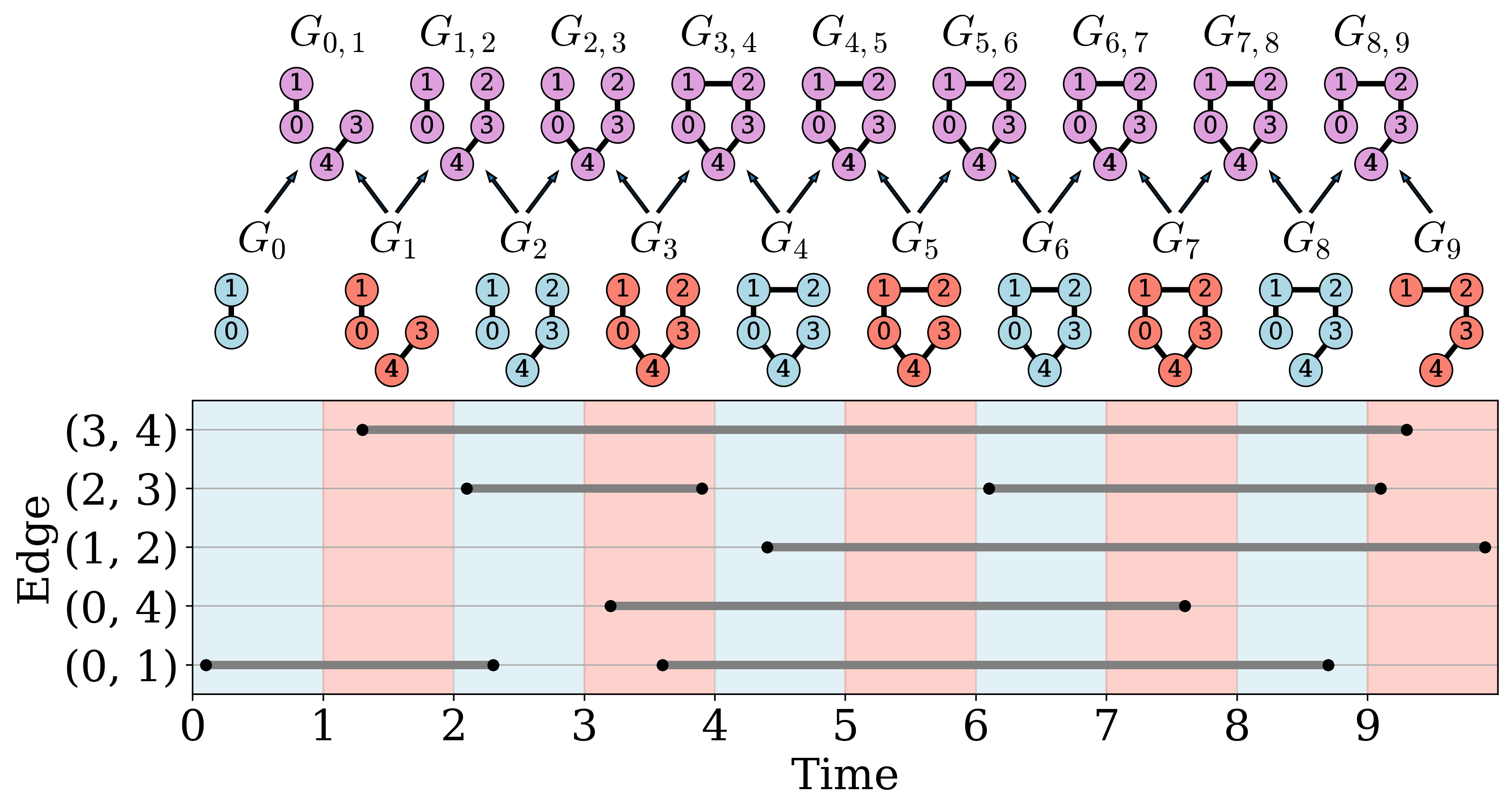
To better understand the resulting persistence diagram, we can visualize the changing structure of the network by looking at the intervals and corresponding graph snapshots. The following figure shows the graph snapshots and the corresponding unions. It is clear that there is a cycle born at graph 3,4 and dissapears at graph 4 correspodning to the persistence pair (4,4.5) and the cycle is born again at graph 5,6 and breaks at graph 8 corresponding to the persistence pair (6,8.5). For more details on this example we direct the user to our publication titled “Temporal Network Analysis Using Zigzag Persistence.”